https://docs.citusdata.com/en/latest/develop/append.html

https://www.citusdata.com/blog/2016/12/15/citus-replication-model-today-and-tomorrow/

本文内容来自citus官方文档，包括一些原文翻译，简略介绍，使用示例等内容。

Abstract

Append distribution is a specialized technique which requires care to use efficiently. Hash distribution is a better choice for most situations.

追加分配是一项需要谨慎有效使用的专门技术。对于大多数情况，散列分布是更好的选择。

While Citus’ most common use cases involve hash data distribution, it can also distribute timeseries data across a variable number of shards by their order in time. This section provides a short reference to loading, deleting, and manipulating timeseries data.

虽然Citus最常见的用例涉及散列数据分布，但它也可以按时间顺序将timeseries数据分布在数量可变的分片上。本节提供有关加载、删除和操作timeseries数据的简短参考。

As the name suggests, append based distribution is more suited to append-only use cases. This typically includes event based data which arrives in a time-ordered series. You can then distribute your largest tables by time, and batch load your events into Citus in intervals of N minutes. This data model can be generalized to a number of time series use cases; for example, each line in a website’s log file, machine activity logs or aggregated website events. Append based distribution supports more efficient range queries. This is because given a range query on the distribution key, the Citus query planner can easily determine which shards overlap that range and send the query only to relevant shards.

顾名思义，基于append的分布更适合仅追加的用例。这通常包括按时间顺序到达的基于事件的数据。然后可以按时间分布最大的表，并以N分钟为间隔将事件批量加载到Citus中。该数据模型可以推广到多个时间序列用例;例如，网站日志文件中的每一行、机器活动日志或聚合的网站事件。基于附加的分布支持更有效的范围查询。这是因为，给定分布键上的范围查询，Citus查询计划器可以很容易地确定哪些分片与该范围重叠，并只将查询发送到相关的分片。

Hash based distribution is more suited to cases where you want to do real-time inserts along with analytics on your data or want to distribute by a non-ordered column (eg. user id). This data model is relevant for real-time analytics use cases; for example, actions in a mobile application, user website events, or social media analytics. In this case, Citus will maintain minimum and maximum hash ranges for all the created shards. Whenever a row is inserted, updated or deleted, Citus will redirect the query to the correct shard and issue it locally. This data model is more suited for doing co-located joins and for queries involving equality based filters on the distribution column.

基于散列的分布更适合于这样的情况，即您希望执行实时插入并对数据进行分析，或者希望按无序列进行分布(例如。用户id)。这个数据模型与实时分析用例相关;例如，移动应用程序中的操作、用户网站事件或社交媒体分析。在这种情况下，Citus将为所有创建的分片维护最小和最大散列范围。无论何时插入、更新或删除一行，Citus都会将查询重定向到正确的分片，并在本地发出它。此数据模型更适合于在分布列上执行协同定位连接和涉及基于等式的过滤器的查询。

Citus uses slightly different syntaxes for creation and manipulation of append and hash distributed tables. Also, the operations supported on the tables differ based on the distribution method chosen. In the sections that follow, we describe the syntax for creating append distributed tables, and also describe the operations which can be done on them.

Citus在创建和操作append和散列分布式表时使用的语法略有不同。此外，根据所选择的分发方法，表上支持的操作也有所不同。在接下来的小节中，我们将描述用于创建append分布式表的语法，并描述可以对其进行的操作。

Creating and Distributing Tables

1
2
3
4
5
6
7
8
9
10
11
12

CREATE TABLE github_events
(
    event_id bigint,
    event_type text,
    event_public boolean,
    repo_id bigint,
    payload jsonb,
    repo jsonb,
    actor jsonb,
    org jsonb,
    created_at timestamp
);

Next, you can use the create_distributed_table() function to mark the table as an append distributed table and specify its distribution column.

接下来，可以使用create_distributed_table()函数将该表标记为追加分布式表并指定其分布列。

1

SELECT create_distributed_table('github_events', 'created_at', 'append');

This function informs Citus that the github_events table should be distributed by append on the created_at column. Note that this method doesn’t enforce a particular distribution; it merely tells the database to keep minimum and maximum values for the created_at column in each shard which are later used by the database for optimizing queries.

该函数通知Citus, github_events表应该通过追加到created_at列上的方式分发。请注意，此方法并不强制执行特定的分发;它只是告诉数据库在每个分片中保留created_at列的最小值和最大值，稍后数据库将使用这些值来优化查询。

Expiring Data

In append distribution, users typically want to track data only for the last few months / years. In such cases, the shards that are no longer needed still occupy disk space. To address this, Citus provides a user defined function master_apply_delete_command() to delete old shards. The function takes a DELETE command as input and deletes all the shards that match the delete criteria with their metadata.

在append分发中，用户通常只想跟踪最近几个月/几年的数据。在这种情况下，不再需要的分片仍然占用磁盘空间。为了解决这个问题，Citus提供了一个用户定义的函数master_apply_delete_command()来删除旧分片。该函数以DELETE命令作为输入，并删除与删除条件匹配的所有分片及其元数据。

The function uses shard metadata to decide whether or not a shard needs to be deleted, so it requires the WHERE clause in the DELETE statement to be on the distribution column. If no condition is specified, then all shards are selected for deletion. The UDF then connects to the worker nodes and issues DROP commands for all the shards which need to be deleted. If a drop query for a particular shard replica fails, then that replica is marked as TO DELETE. The shard replicas which are marked as TO DELETE are not considered for future queries and can be cleaned up later.

该函数使用分片元数据来决定是否需要删除分片，因此它要求DELETE语句中的WHERE子句位于分布列上。如果没有指定任何条件，则选择删除所有分片。然后，UDF连接到工作节点，并发出删除所有需要删除的分片的命令。如果针对特定分片副本的drop查询失败，则该副本被标记为要删除。标记为要删除的shard副本不会考虑用于将来的查询，可以在以后进行清理。

The example below deletes those shards from the github_events table which have all rows with created_at >= ‘2015-01-01 00:00:00’. Note that the table is distributed on the created_at column.

下面的示例将从github_events表中删除那些包含created_at >= ‘ 2015-01-01 00:00:00 ‘的所有行。注意，表分布在created_at列上。

1
2
3
4
5

SELECT * from master_apply_delete_command('DELETE FROM github_events WHERE created_at >= ''2015-01-01 00:00:00''');
 master_apply_delete_command
-----------------------------
                           3
(1 row)

To learn more about the function, its arguments and its usage, please visit the Citus Utility Functions section of our documentation. Please note that this function only deletes complete shards and not individual rows from shards. If your use case requires deletion of individual rows in real-time, see the section below about deleting data.

请注意，此函数只删除完整的分片，而不删除分片中的单个行。如果您的用例需要实时删除个别行，请参阅下面关于删除数据的部分。

Deleting Data

The most flexible way to modify or delete rows throughout a Citus cluster with regular SQL statements:

最灵活的方式来修改或删除整个Citus集群的常规SQL语句行:

1
2

DELETE FROM github_events
WHERE created_at >= '2015-01-01 00:03:00';

Unlike master_apply_delete_command, standard SQL works at the row- rather than shard-level to modify or delete all rows that match the condition in the where clause. It deletes rows regardless of whether they comprise an entire shard.

与master_apply_delete_command不同，标准SQL在行上工作，而不是在分片级上修改或删除与where子句中的条件匹配的所有行。它删除行，不管它们是否包含整个分片。

Dropping Tables

You can use the standard PostgreSQL DROP TABLE command to remove your append distributed tables. As with regular tables, DROP TABLE removes any indexes, rules, triggers, and constraints that exist for the target table. In addition, it also drops the shards on the worker nodes and cleans up their metadata.

可以使用标准的PostgreSQL DROP TABLE命令删除附加的分布式表。与常规表一样，DROP表删除目标表的所有索引、规则、触发器和约束。此外，它还删除工作节点上的分片并清理它们的元数据。

1

DROP TABLE github_events;

Data Loading

Citus supports two methods to load data into your append distributed tables. The first one is suitable for bulk loads from files and involves using the \copy command. For use cases requiring smaller, incremental data loads, Citus provides two user defined functions. We describe each of the methods and their usage below.

Citus支持两种方法来将数据加载到附加的分布式表中。第一种方法适用于从文件进行批量加载，并涉及到使用\copy命令。对于需要更小的增量数据负载的用例，Citus提供了两个用户定义的函数。我们将在下面描述每种方法及其用法。

Bulk load using \copy

The \copy command is used to copy data from a file to a distributed table while handling replication and failures automatically. You can also use the server side COPY command. In the examples, we use the \copy command from psql, which sends a COPY .. FROM STDIN to the server and reads files on the client side, whereas COPY from a file would read the file on the server.

[\copy](http://www.postgresql.org/docs/current/static/app-psql.html# app-psql - metadata - copy)命令用于将数据从文件复制到分布式表，同时自动处理复制和失败。您还可以使用服务器端COPY命令。在本例中，我们使用来自psql的\copy命令，它发送一个副本…从STDIN到服务器并读取客户端上的文件，而从文件复制则读取服务器上的文件。

You can use \copy both on the coordinator and from any of the workers. When using it from the worker, you need to add the master_host option. Behind the scenes, \copy first opens a connection to the coordinator using the provided master_host option and uses master_create_empty_shard to create a new shard. Then, the command connects to the workers and copies data into the replicas until the size reaches shard_max_size, at which point another new shard is created. Finally, the command fetches statistics for the shards and updates the metadata.

您可以在协调节点和任何工作节点上使用\copy。当从工作节点中使用它时，您需要添加master_host选项。在后台，\copy首先使用提供的master_host选项打开到协调节点的连接，并使用master_create_empty_shard创建一个新的shard。然后，该命令连接到工作节点并将数据复制到副本中，直到大小达到shard_max_size，此时将创建另一个新分片。最后，该命令获取分片的统计信息并更新元数据。

1
2

SET citus.shard_max_size TO '64MB';
\copy github_events from 'github_events-2015-01-01-0.csv' WITH (format CSV, master_host 'coordinator-host')

Citus assigns a unique shard id to each new shard and all its replicas have the same shard id. Each shard is represented on the worker node as a regular PostgreSQL table with name ‘tablename_shardid’ where tablename is the name of the distributed table and shardid is the unique id assigned to that shard. One can connect to the worker postgres instances to view or run commands on individual shards.

Citus分配一个惟一的分片id到每个新分片及其所有副本具有相同的分片id。每个分片是工人代表节点作为常规PostgreSQL表名称的tablename_shardid分布表的表名是名字的和shardid是惟一的id分配到分片。可以连接到worker postgres实例来查看或运行单个分片上的命令。

By default, the \copy command depends on two configuration parameters for its behavior. These are called citus.shard_max_size and citus.shard_replication_factor.

默认情况下，\copy命令的行为取决于两个配置参数。分别是：citus.shard_max_size 和citus.shard_replication_factor

1. citus.shard_max_size :- This parameter determines the maximum size of a shard created using \copy, and defaults to 1 GB. If the file is larger than this parameter, \copy will break it up into multiple shards.
2. 此参数确定使用\copy创建的分片的最大大小，默认为1 GB。如果文件比这个参数大，\copy将把它分成多个分片。
3. citus.shard_replication_factor :- This parameter determines the number of nodes each shard gets replicated to, and defaults to one. Set it to two if you want Citus to replicate data automatically and provide fault tolerance. You may want to increase the factor even higher if you run large clusters and observe node failures on a more frequent basis.
4. 该参数决定每个shard复制到的节点数量，默认为一个。如果希望Citus自动复制数据并提供容错，请将其设置为2。如果您运行大型集群并更频繁地观察节点故障，则可能希望进一步提高这个因素。

The configuration setting citus.shard_replication_factor can only be set on the coordinator node.

配置设置citus。shard_replication_factor只能在协调节点上设置。

Please note that you can load several files in parallel through separate database connections or from different nodes. It is also worth noting that \copy always creates at least one shard and does not append to existing shards. You can use the method described below to append to previously created shards.

请注意，您可以通过单独的数据库连接或从不同的节点并行加载多个文件。还值得注意的是，\copy总是创建至少一个切分，并且不会附加到现有的切分上。您可以使用下面描述的方法将之前创建的分片追加到后面。

There is no notion of snapshot isolation across shards, which means that a multi-shard SELECT that runs concurrently with a COPY might see it committed on some shards, but not on others. If the user is storing events data, he may occasionally observe small gaps in recent data. It is up to applications to deal with this if it is a problem (e.g. exclude the most recent data from queries, or use some lock).

没有跨分片的快照隔离的概念，这意味着与一个副本并发运行的多分片选择可能会在一些分片上提交，而不是在其他分片上提交。如果用户正在存储事件数据，他可能会偶尔观察到最近数据中的小间隙。如果这是一个问题，则由应用程序来处理(例如，从查询中排除最近的数据，或使用一些锁)。

If COPY fails to open a connection for a shard placement then it behaves in the same way as INSERT, namely to mark the placement(s) as inactive unless there are no more active placements. If any other failure occurs after connecting, the transaction is rolled back and thus no metadata changes are made.

如果复制无法为分片放置打开连接，那么它的行为与INSERT相同，即将放置标记为非活动的，除非没有更多的活动放置。如果连接后发生任何其他故障，则事务将回滚，因此不会对元数据进行更改。

Incremental loads by appending to existing shards

The \copy command always creates a new shard when it is used and is best suited for bulk loading of data. Using \copy to load smaller data increments will result in many small shards which might not be ideal. In order to allow smaller, incremental loads into append distributed tables, Citus provides 2 user defined functions. They are master_create_empty_shard() and master_append_table_to_shard().

当使用\copy命令时，它总是创建一个新的分片，并且最适合批量加载数据。使用\copy加载较小的数据增量将导致许多小分片，这可能不是理想的结果。为了允许向append分布式表中增加更小的负载，Citus提供了两个用户定义的函数。它们是master_create_empty_shard()和master_append_table_to_shard()。

master_create_empty_shard() can be used to create new empty shards for a table. This function also replicates the empty shard to citus.shard_replication_factor number of nodes like the \copy command.

master_create_empty_shard()可用于为表创建新的空分片。此函数还将空分片复制到citus。shard_replication_factor节点数，如\copy命令。

master_append_table_to_shard() can be used to append the contents of a PostgreSQL table to an existing shard. This allows the user to control the shard to which the rows will be appended. It also returns the shard fill ratio which helps to make a decision on whether more data should be appended to this shard or if a new shard should be created.

master_append_table_to_shard()可用于将PostgreSQL表的内容附加到现有的shard。这允许用户控制将附加行的分片。它还返回分片填充率，这有助于决定是否应该向这个分片添加更多的数据，还是应该创建一个新的分片。

To use the above functionality, you can first insert incoming data into a regular PostgreSQL table. You can then create an empty shard using master_create_empty_shard(). Then, using master_append_table_to_shard(), you can append the contents of the staging table to the specified shard, and then subsequently delete the data from the staging table. Once the shard fill ratio returned by the append function becomes close to 1, you can create a new shard and start appending to the new one.

要使用上述功能，您可以首先将传入的数据插入到常规的PostgreSQL表中。然后可以使用master_create_empty_shard()创建一个空分片。然后，使用master_append_table_to_shard()，可以将staging表的内容附加到指定的shard中，然后从staging表中删除数据。一旦append函数返回的分片填充比接近1，您就可以创建一个新的分片并开始将其附加到新的分片中。

1
2
3
4
5
6
7
8
9
10
11

SELECT * from master_create_empty_shard('github_events');
master_create_empty_shard
---------------------------
                102089
(1 row)

SELECT * from master_append_table_to_shard(102089, 'github_events_temp', 'master-101', 5432);
master_append_table_to_shard
------------------------------
        0.100548
(1 row)

To learn more about the two UDFs, their arguments and usage, please visit the Citus Utility Functions section of the documentation.

Example

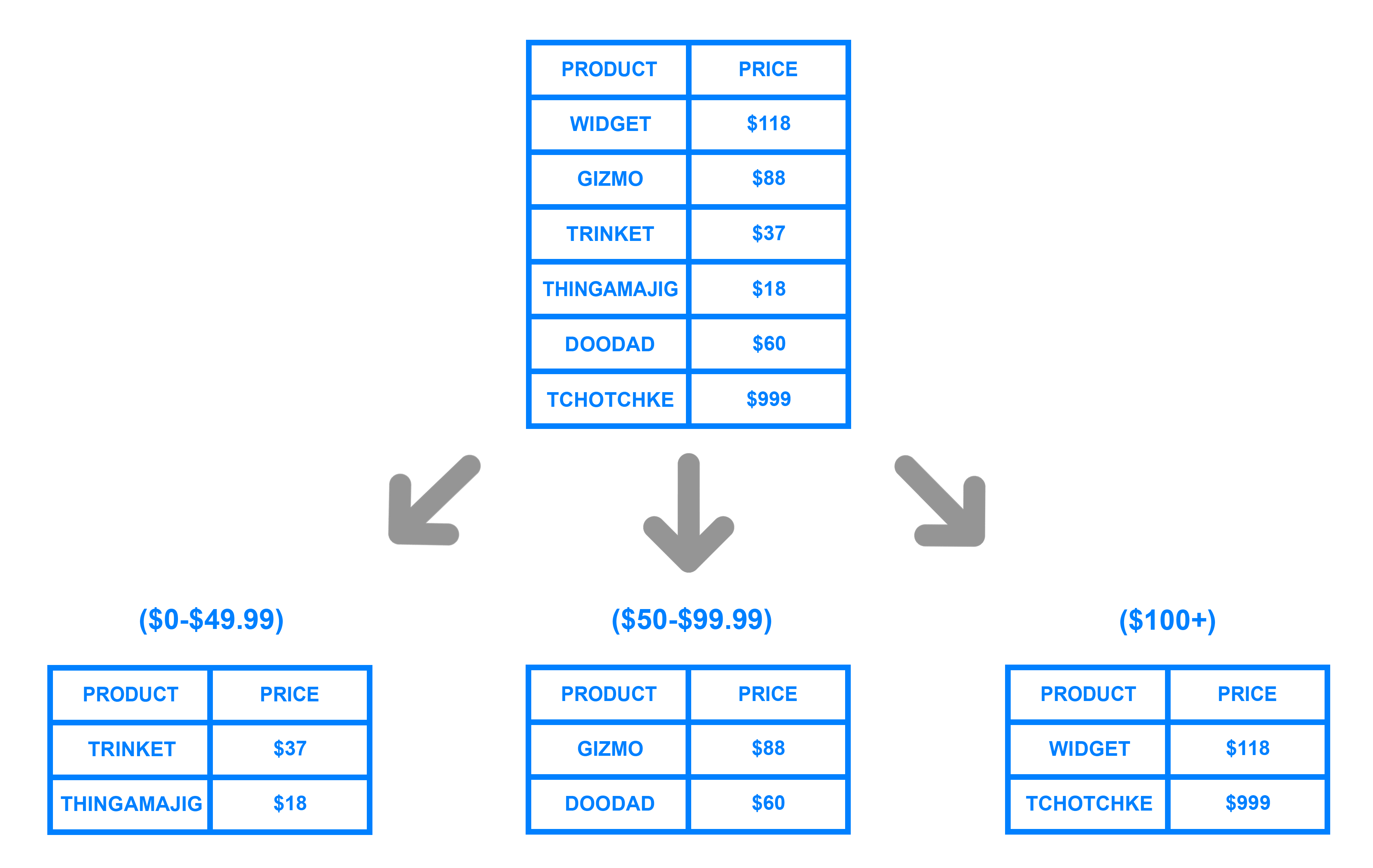
Range Based Sharding

1
2
3
4
5
6
7
8
9
10
11
12
13
14
15
16
17
18
19
20
21
22
23
24
25
26
27
28
29
30
31
32
33
34
35
36
37
38
39
40
41
42
43
44
45
46
47
48
49
50
51
52
53
54
55
56
57
58
59
60
61
62
63
64
65
66
67
68
69
70
71
72
73
74
75
76
77
78
79
80
81
82
83
84
85
86
87
88
89
90
91
92
93
94
95
96
97
98
99
100
101
102
103
104
105
106
107
108
109
110
111
112
113
114
115
116

young=# create table test(id int, ts timestamptz);
CREATE TABLE
young=# SELECT create_distributed_table('test', 'ts', 'append');
NOTICE:  using statement-based replication
DETAIL:  Streaming replication is supported only for hash-distributed tables.
 create_distributed_table 
--------------------------
 
(1 row)

young=# SELECT * from master_create_empty_shard('test');
 master_create_empty_shard 
---------------------------
                    102046
(1 row)

young=# insert into test values (1, now());
INSERT 0 1
young=# table test ;
 id |              ts               
----+-------------------------------
  1 | 2019-11-07 15:02:23.850578+08
(1 row)

young=# table pg_dist_shard;
 logicalrelid | shardid | shardstorage | shardminvalue | shardmaxvalue 
--------------+---------+--------------+---------------+---------------
 test         |  102046 | t            |               | 
(1 row)

young=# insert into test values (2, now());
INSERT 0 1
young=# SELECT                             
    n.nodename,
    n.nodeport,
    sum(foo.result::int4)
FROM (
    SELECT *
    FROM
        run_command_on_shards ('test',
            'select count(*) from %s')) AS foo,
    pg_dist_placement p,
    pg_dist_node n
WHERE
    foo.shardid = p.shardid
    AND p.groupid = n.groupid
GROUP BY
    n.nodename,
    n.nodeport;
 nodename | nodeport | sum 
----------+----------+-----
 10.0.0.5 |     9432 |   2
(1 row)

young=# SELECT * from master_create_empty_shard('test');
 master_create_empty_shard 
---------------------------
                    102047
(1 row)

young=# insert into test values (3, now());             
ERROR:  cannot run INSERT command which targets multiple shards
HINT:  Make sure the value for partition column "ts" falls into a single shard.
young=# table pg_dist_shard;
 logicalrelid | shardid | shardstorage | shardminvalue | shardmaxvalue 
--------------+---------+--------------+---------------+---------------
 test         |  102046 | t            |               | 
 test         |  102047 | t            |               | 
(2 rows)

young=# select min(ts), max(ts) from test;
              min              |              max              
-------------------------------+-------------------------------
 2019-11-07 15:02:23.850578+08 | 2019-11-07 15:03:46.776405+08
(1 row)

young=# update pg_dist_shard set shardminvalue = '2019-11-07 15:00:00', shardmaxvalue = '2019-11-07 15:04:59' where shardid = 102046;
UPDATE 1
young=# table pg_dist_shard;
 logicalrelid | shardid | shardstorage |    shardminvalue    |    shardmaxvalue    
--------------+---------+--------------+---------------------+---------------------
 test         |  102047 | t            |                     | 
 test         |  102046 | t            | 2019-11-07 15:00:00 | 2019-11-07 15:04:59
(2 rows)

young=# SELECT                                          
    n.nodename,
    n.nodeport,
    sum(foo.result::int4)
FROM (
    SELECT *
    FROM
        run_command_on_shards ('test',
            'select count(*) from %s')) AS foo,
    pg_dist_placement p,
    pg_dist_node n
WHERE
    foo.shardid = p.shardid
    AND p.groupid = n.groupid
GROUP BY
    n.nodename,
    n.nodeport;
 nodename  | nodeport | sum 
-----------+----------+-----
 10.0.0.5  |     9432 |   2
 10.0.0.10 |     9432 |   1
(2 rows)

young=# update pg_dist_shard set shardminvalue = '2019-11-07 15:05:00', shardmaxvalue = '2019-11-07 15:09:59' where shardid = 102047;
UPDATE 1
young=# table pg_dist_shard;
 logicalrelid | shardid | shardstorage |    shardminvalue    |    shardmaxvalue    
--------------+---------+--------------+---------------------+---------------------
 test         |  102046 | t            | 2019-11-07 15:00:00 | 2019-11-07 15:04:59
 test         |  102047 | t            | 2019-11-07 15:05:00 | 2019-11-07 15:09:59
(2 rows)

文档有介绍删除分片、删除数据及删除表，未介绍TRUNCATE

1
2
3
4
5
6
7
8
9
10
11
12

young=# table pg_dist_shard;
 logicalrelid | shardid | shardstorage |    shardminvalue    |    shardmaxvalue    
--------------+---------+--------------+---------------------+---------------------
 test         |  102046 | t            | 2019-11-07 15:00:00 | 2019-11-07 15:04:59
 test         |  102047 | t            | 2019-11-07 15:05:00 | 2019-11-07 15:09:59
(2 rows)
young=# truncate test ;
TRUNCATE TABLE
young=# table pg_dist_shard;
 logicalrelid | shardid | shardstorage | shardminvalue | shardmaxvalue 
--------------+---------+--------------+---------------+---------------
(0 rows)

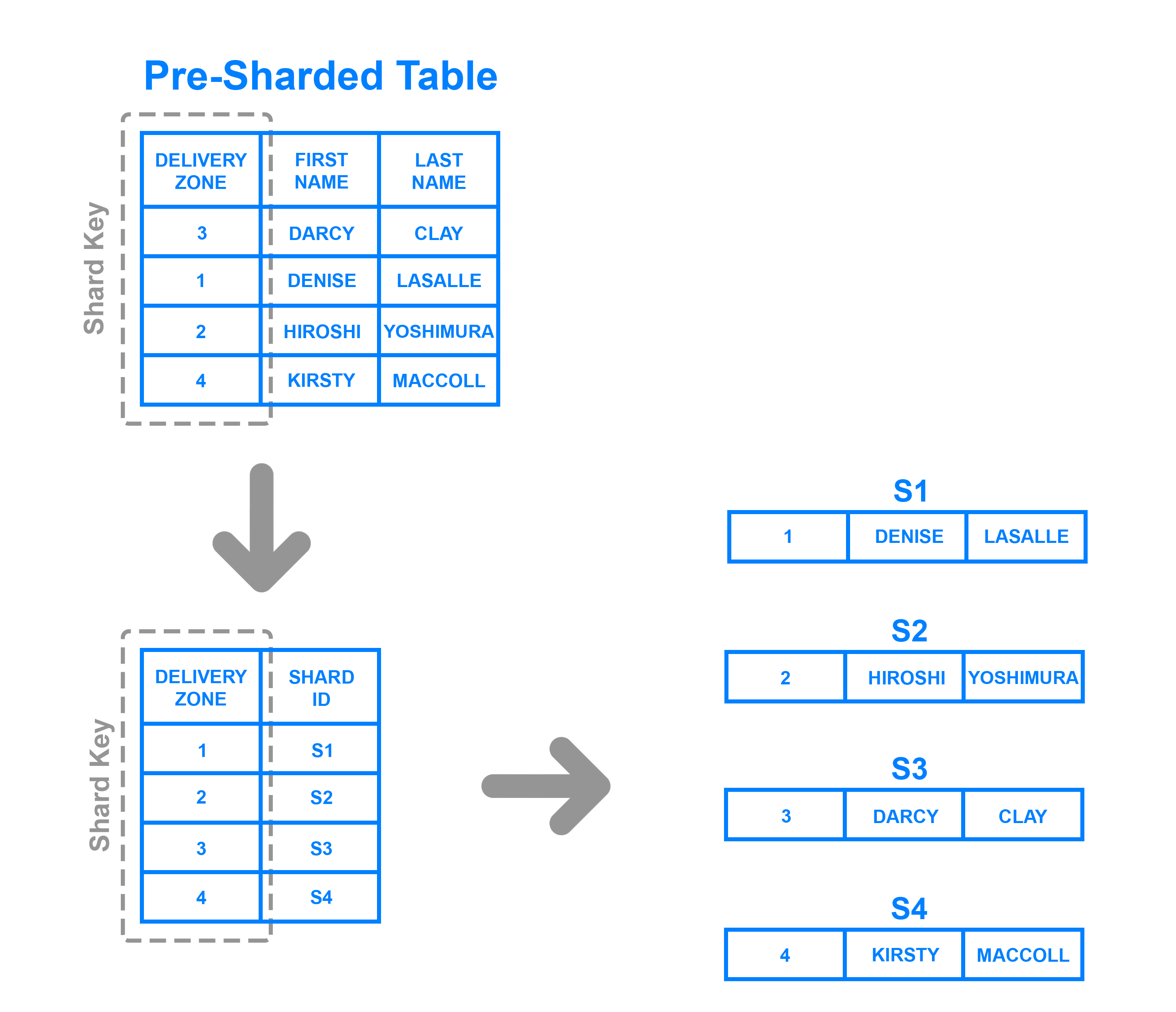
Directory Based Sharding

这与基于范围的分片类似，但不是确定分片键的数据属于哪个范围，而是将每个键绑定到其自己的特定分片。

1
2
3
4
5
6
7
8
9
10
11
12
13
14
15
16
17
18
19
20
21
22
23
24
25
26
27
28
29
30
31
32
33
34

young=# create table list(id int, col text);
CREATE TABLE
young=# SELECT create_distributed_table('list', 'col', 'append');
NOTICE:  using statement-based replication
DETAIL:  Streaming replication is supported only for hash-distributed tables.
 create_distributed_table 
--------------------------
 
(1 row)

young=# select master_create_empty_shard('list');
 master_create_empty_shard 
---------------------------
                    102052
(1 row)

young=# update pg_dist_shard set shardminvalue = 'beijing', shardmaxvalue = 'beijing' where shardid = 102052;
UPDATE 1
young=# table pg_dist_shard;
 logicalrelid | shardid | shardstorage | shardminvalue | shardmaxvalue 
--------------+---------+--------------+---------------+---------------
 list         |  102052 | t            | beijing       | beijing
(1 row)

young=# insert into list values (1, 'beijing');
INSERT 0 1
young=# insert into list values (2, 'hangzhou');
ERROR:  cannot run INSERT command which targets no shards
HINT:  Make sure you have created a shard which can receive this partition column value.
young=# table list ;
 id |   col   
----+---------
  1 | beijing
(1 row)

bulk load using copy

大小达到shard_max_size，将创建另一个新分片

此示例中一个copy创建多个分片

1
2
3
4
5
6
7
8
9
10
11
12
13
14
15
16
17
18
19
20
21
22
23
24
25
26
27
28
29
30
31
32
33
34
35
36
37
38
39
40
41
42
43
44
45
46
47
48
49
50
51
52
53
54
55
56
57
58
59
60
61
62
63
64
65
66
67
68
69
70
71
72
73
74
75
76
77
78
79
80
81
82
83
84
85
86
87

young=# show citus.shard_max_size ;
 citus.shard_max_size 
----------------------
 1GB
(1 row)

young=# table pg_dist_shard;
 logicalrelid | shardid | shardstorage | shardminvalue | shardmaxvalue 
--------------+---------+--------------+---------------+---------------
(0 rows)

young=# \copy github_events from '/data/citus/github_events-2015-01-01-0.csv' WITH (format CSV);
COPY 7702

young=# SELECT                                                                                  
    n.nodename,
    n.nodeport,
    sum(foo.result::int4)
FROM (
    SELECT *
    FROM
        run_command_on_shards ('github_events',
            'select count(*) from %s')) AS foo,
    pg_dist_placement p,
    pg_dist_node n
WHERE
    foo.shardid = p.shardid
    AND p.groupid = n.groupid
GROUP BY
    n.nodename,
    n.nodeport;
 nodename  | nodeport | sum  
-----------+----------+------
 10.0.0.20 |     9432 | 7702
(1 row)

young=# table pg_dist_shard;
 logicalrelid  | shardid | shardstorage |    shardminvalue    |    shardmaxvalue    
---------------+---------+--------------+---------------------+---------------------
 github_events |  102053 | t            | 2015-01-01 00:00:00 | 2015-01-01 00:59:58
(1 row)

young=# SET citus.shard_max_size TO '4MB';
SET
young=# show citus.shard_max_size ;
 citus.shard_max_size 
----------------------
 4MB
(1 row)

young=# \copy github_events from '/data/citus/github_events-2015-01-01-1.csv' WITH (format CSV);
COPY 7427
young=# table pg_dist_shard;
 logicalrelid  | shardid | shardstorage |    shardminvalue    |    shardmaxvalue    
---------------+---------+--------------+---------------------+---------------------
 github_events |  102053 | t            | 2015-01-01 00:00:00 | 2015-01-01 00:59:58
 github_events |  102054 | t            | 2015-01-01 01:00:00 | 2015-01-01 01:14:55
 github_events |  102055 | t            | 2015-01-01 01:14:55 | 2015-01-01 01:27:40
 github_events |  102056 | t            | 2015-01-01 01:27:40 | 2015-01-01 01:41:02
 github_events |  102057 | t            | 2015-01-01 01:41:02 | 2015-01-01 01:56:29
 github_events |  102058 | t            | 2015-01-01 01:56:29 | 2015-01-01 01:59:59
(6 rows)

young=# SELECT              
    n.nodename,
    n.nodeport,
    sum(foo.result::int4)
FROM (
    SELECT *
    FROM
        run_command_on_shards ('github_events',
            'select count(*) from %s')) AS foo,
    pg_dist_placement p,
    pg_dist_node n
WHERE
    foo.shardid = p.shardid
    AND p.groupid = n.groupid
GROUP BY
    n.nodename,
    n.nodeport;
 nodename  | nodeport | sum  
-----------+----------+------
 10.0.0.20 |     9432 | 9506
 10.0.0.5  |     9432 | 2300
 10.0.0.10 |     9432 | 1662
 10.0.0.21 |     9432 | 1661
(4 rows)

appending to existing shards

1
2
3
4
5
6
7
8
9
10
11
12
13
14
15
16
17
18
19
20
21
22
23
24
25
26
27
28
29
30
31
32
33
34
35
36
37
38
39
40
41
42
43
44
45
46
47
48
49
50
51

young=# create table test(id int , col int);
CREATE TABLE
young=# SELECT create_distributed_table('test', 'col', 'append');
NOTICE:  using statement-based replication
DETAIL:  Streaming replication is supported only for hash-distributed tables.
 create_distributed_table 
--------------------------
 
(1 row)

young=# create table tmp (id int, col int);
CREATE TABLE
young=# insert into tmp select id, id from generate_series(1,5) as id;
INSERT 0 5
young=# table tmp ;
 id | col 
----+-----
  1 |   1
  2 |   2
  3 |   3
  4 |   4
  5 |   5
(5 rows)

young=# select master_create_empty_shard('test');
 master_create_empty_shard 
---------------------------
                    102059
(1 row)

young=# SELECT master_append_table_to_shard(102059, 'tmp', '10.0.0.4', 9432);
 master_append_table_to_shard 
------------------------------
                   0.00195312
(1 row)

young=# table pg_dist_shard;
 logicalrelid  | shardid | shardstorage |    shardminvalue    |    shardmaxvalue    
---------------+---------+--------------+---------------------+---------------------
 test          |  102059 | t            | 1                   | 5
(1 rows)

young=# table test ;
 id | col 
----+-----
  1 |   1
  2 |   2
  3 |   3
  4 |   4
  5 |   5
(5 rows)

other

ERROR: cannot run INSERT command which targets multiple shards

1
2
3
4
5
6
7
8
9
10
11
12
13
14
15
16
17
18
19
20
21
22
23
24
25
26
27
28
29
30
31
32
33
34
35
36
37
38
39

cat test.csv 
1,1
2,2
3,3
4,4
5,5

young=# copy test from '/data/citus/test.csv' with csv;
COPY 5
young=# table pg_dist_shard;
 logicalrelid  | shardid | shardstorage |    shardminvalue    |    shardmaxvalue    
---------------+---------+--------------+---------------------+---------------------
 test          |  102096 | t            | 1                   | 5
(1 rows)

cat test.csv 
7,7
8,8
young=# copy test from '/data/citus/test.csv' with csv;
COPY 2
young=# table pg_dist_shard;
 logicalrelid  | shardid | shardstorage |    shardminvalue    |    shardmaxvalue    
---------------+---------+--------------+---------------------+---------------------
 test          |  102096 | t            | 1                   | 5
 test          |  102097 | t            | 7                   | 8
(2 rows)

cat test.csv 
8,8
9,9
young=# copy test from '/data/citus/test.csv' with csv;
COPY 2
young=# table pg_dist_shard;
 logicalrelid  | shardid | shardstorage |    shardminvalue    |    shardmaxvalue    
---------------+---------+--------------+---------------------+---------------------
 test          |  102096 | t            | 1                   | 5
 test          |  102097 | t            | 7                   | 8
 test          |  102098 | t            | 8                   | 9
(3 rows)

shard_102097和shard_102098分区边界重合

1
2
3
4
5
6
7
8
9
10
11
12
13
14
15
16
17
18
19
20
21
22
23
24
25
26
27

young=# SELECT
    n.nodename,
    n.nodeport,
    sum(foo.result::int4)
FROM (
    SELECT *
    FROM
        run_command_on_shards ('test',
            'select count(*) from %s')) AS foo,
    pg_dist_placement p,
    pg_dist_node n
WHERE
    foo.shardid = p.shardid
    AND p.groupid = n.groupid
GROUP BY
    n.nodename,
    n.nodeport;
 nodename  | nodeport | sum 
-----------+----------+-----
 10.0.0.20 |     9432 |   2
 10.0.0.5  |     9432 |   2
 10.0.0.21 |     9432 |   5
(3 rows)

young=# insert into test values (8,8);
ERROR:  cannot run INSERT command which targets multiple shards
HINT:  Make sure the value for partition column "col" falls into a single shard.

ERROR: INSERT … SELECT into an append-distributed table is not supported

1
2
3
4
5
6
7
8
9
10

young=# table pg_dist_shard;
 logicalrelid | shardid | shardstorage |    shardminvalue    |    shardmaxvalue    
--------------+---------+--------------+---------------------+---------------------
 range        |  102050 | t            | 11                  | 15
 range        |  102049 | t            | 6                   | 10
 range        |  102048 | t            | 0                   | 5
(3 rows)

young=# insert into range select id, id from generate_series(1,15) as id;
ERROR:  INSERT ... SELECT into an append-distributed table is not supported

replication model

以append方式建表时可以注意到

1
2

NOTICE:  using statement-based replication
DETAIL:  Streaming replication is supported only for hash-distributed tables.

citus 有两种复制模式：基于语句复制、流复制

最初版本的citus主要用来做实时分析，数据也是通过追加方式存储在分布式集群中。

事件数据的这些属性使事件数据的并行加载变得相对容易，而不需要牺牲一致性语义。协调节点将保存与集群中的分片和分片放置(副本)相关的元数据。然后，客户机将与协调节点节点通信，并交换元数据，以便在这些元数据上附加事件数据分片。一旦客户端将相关事件数据附加到相关分片中，客户端将通过更新协调节点上的分片元数据来结束操作。

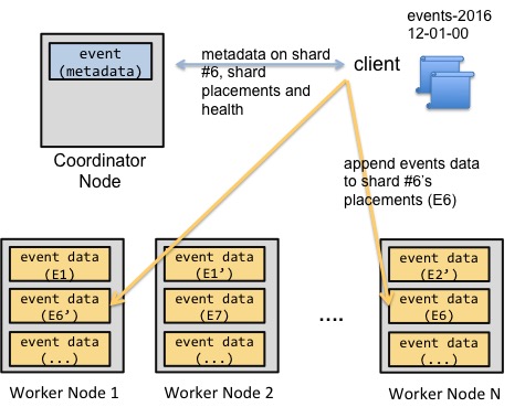
上面的简化图显示了一个数据加载示例。客户端告诉协调节点节点，它希望将事件数据追加到追加分布式表中。协调节点向客户提供有关shard 6的位置信息。然后客户端将这些事件复制到分片的位置，并使用相关元数据更新协调节点。如果客户机无法将事件复制到其中一个节点，它可以将相关分片的位置标记为无效，也可以中止复制操作。

追加分配还存在一个问题是不能更新数据，上面已经做过测试。

因此，我们将Citus的基于语句的复制模型进行了扩展。 在该模型中，我们还提供了哈希分布作为一种数据分布方法。通过这种方式，用户可以轻松地更新和删除单独的行。启用更新和删除还需要解决两个问题:更新同一行的并发客户机，以及在更新期间一个shard副本不可用。

因此，我们以两种方式扩展了协调节点。首先，协调节点处理涉及相同分片的update和delete语句的锁定。其次，如果协调节点在写操作期间无法到达分片副本，则会将该副本标记为不健康。然后，用户将运行一个命令来修复不健康的副本。

从一致性语义的角度来看，这种方法通常称为读写一致性（写后读一致性）。

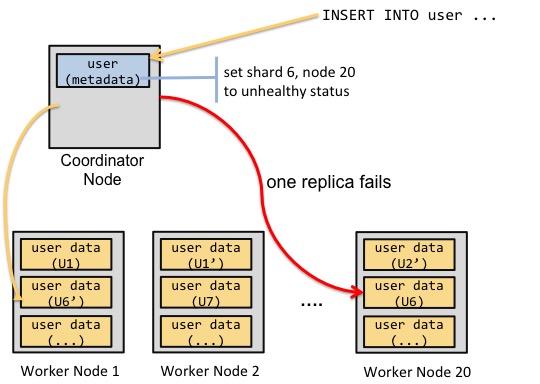
假设您有200个表，如果并发更新了10个表的分片，但是无法到达保存分片副本的机器您需要将该机器上的所有200个分片副本标记为非活动的。

如果高可用性特性，那么基于语句的复制通常是不够好的。

解决方法之一是将 replication factor 设置为1，不使用副本。

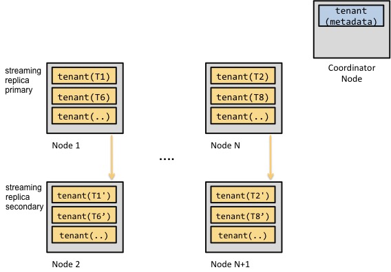
另一种方案是从基于语句复制切换到流复制。

这种方法的架构如下：

简介

相同sql，limit 1和limit 10，走不同索引，效率相差很大

实际执行计划如下:

1
2
3
4
5
6
7
8
9
10
11
12
13
14
15
16
17
18
19
20
21
22
23

test=# explain analyze select data_id from test_tbl where status=0 and city_id=310188 and type=103 and sub_type in(10306,10304,10305) order by create_time desc limit 1;
                                                                                    QUERY PLAN                                                                                   
----------------------------------------------------------------------------------------------------------------------------------------------------------------------------------
 Limit  (cost=0.44..1690.33 rows=1 width=16) (actual time=12816.268..12816.269 rows=1 loops=1)
   ->  Index Scan Backward using test_tbl_create_time_idx on test_tbl  (cost=0.44..1936615.36 rows=1146 width=16) (actual time=12816.266..12816.266 rows=1 loops=1)
         Filter: ((status = 0) AND (city_id = 310188) AND (type = 103) AND (sub_type = ANY ('{10306,10304,10305}'::integer[])))
         Rows Removed by Filter: 9969343
 Planning time: 2.940 ms
 Execution time: 12816.306 ms
(6 rows)
 
test=# explain analyze select data_id from test_tbl where status=0 and city_id=310188 and type=103 and sub_type in(10306,10304,10305) order by create_time desc limit 10;
                                                                                      QUERY PLAN                                                                                     
--------------------------------------------------------------------------------------------------------------------------------------------------------------------------------------
 Limit  (cost=4268.71..4268.73 rows=10 width=16) (actual time=0.082..0.084 rows=10 loops=1)
   ->  Sort  (cost=4268.71..4271.57 rows=1146 width=16) (actual time=0.082..0.083 rows=10 loops=1)
         Sort Key: create_time
         Sort Method: quicksort  Memory: 25kB
         ->  Index Scan using test_tbl_city_id_sub_type_create_time_idx on test_tbl  (cost=0.44..4243.94 rows=1146 width=16) (actual time=0.030..0.066 rows=15 loops=1)
               Index Cond: ((city_id = 310188) AND (sub_type = ANY ('{10306,10304,10305}'::integer[])))
 Planning time: 0.375 ms
 Execution time: 0.150 ms
(8 rows)

两个走的索引不一样

1
2
3
4
5
6
7
8
9
10
11
12
13
14
15
16

test=# \d test_tbl_create_time_idx
     Index "public.test_tbl_create_time_idx"
   Column    |            Type             | Definition 
-------------+-----------------------------+-------------
 create_time | timestamp without time zone | create_time
btree, for table "public.test_tbl"
 
 
test=# \d test_tbl_city_id_sub_type_create_time_idx
Index "public.test_tbl_city_id_sub_type_create_time_idx"
   Column    |            Type             | Definition 
-------------+-----------------------------+-------------
 city_id     | integer                     | city_id
 sub_type    | integer                     | sub_type
 create_time | timestamp without time zone | create_time
btree, for table "public.test_tbl", predicate (type = 103 AND status = 0)

首先，表的记录数(3123万)除以满足whereclase的记录数(1199)，得到平均需要扫描多少条记录，可以得到一条满足whereclase条件的记录

1
2
3
4
5
6
7
8
9
10
11

test=# select count(*) from test_tbl;
  count  
----------
 31227936
(1 row)
 
test=# select 31227936/1199;
 ?column?
----------
    26044
(1 row)

也就是说每扫描26044条记录，可以得到一条满足条件的记录。（优化器这么算，是认为数据分布是均匀的。）

但是，实际上，数据分布是不均匀的，whereclause的记录在表的前端。

并不是估算的每扫描26044条记录，可以得到一条满足条件的记录。

问题就出在这里。

1
2
3
4
5
6
7
8
9
10
11
12
13
14
15
16
17
18
19
20
21
22
23
24
25
26
27
28
29
30
31
32
33
34

# ctid
test=# select max(ctid) from test_tbl;
     max     
--------------
 (244118,407)
(1 row)
 
test=# select max(ctid),min(ctid) from test_tbl where data_id in (select data_id from test_tbl where status=0 and city_id=310188 and type=103 and sub_type in(10306,10304,10305));
    max     |    min   
------------+-----------
 (21293,15) | (2444,73)
(1 row)
 
 
 
# 分布在28w个rows里(不一定均匀分布),且通过数据分布分别在表中的 page min号 是 2444, max号是21293, 整个表的最大page号是 244118, 可以看出符合条件的28w行,物理分布于表的前端.
 
test=# select 31227936/244118*21293;
 ?column?
----------
  2704211
(1 row)
 
# order by asc 就能看出效果
test=# explain analyze select data_id from test_tbl where status=0 and city_id=310188 and type=103 and sub_type in(10306,10304,10305) order by create_time asc limit 1;
                                                                              QUERY PLAN                                                                              
-----------------------------------------------------------------------------------------------------------------------------------------------------------------------
 Limit  (cost=0.44..1615.86 rows=1 width=16) (actual time=4295.865..4295.866 rows=1 loops=1)
   ->  Index Scan using test_tbl_create_time_idx on test_tbl  (cost=0.44..1936888.15 rows=1199 width=16) (actual time=4295.864..4295.864 rows=1 loops=1)
         Filter: ((status = 0) AND (city_id = 310188) AND (type = 103) AND (sub_type = ANY ('{10306,10304,10305}'::integer[])))
         Rows Removed by Filter: 4712758
 Planning time: 0.404 ms
 Execution time: 4295.884 ms
(6 rows)

为什么走不同的索引

实际上PG会通过计算成本得到应该使用哪个索引

在limit10 时, 使用test_tbl_city_id_sub_type_create_time_idx索引的时候，需要扫描1199行，然后排序，总cost是 cost=4268.71..4271.57，然后取出 desc 的10个tuple,需要的cost是cost=4268.71..4268.73,

实际的执行时间是: actual time=0.082..0.084，从这点来看，limit 10 的真正执行时间比执行计划还快, 可以认为是查询规化器从诸多查询路径中，找到较优的执行计划了.

在 limit 1 时, 使用 test_tbl_create_time_idx的时候,

Limit (cost=0.44..1690.33 rows=1 width=16) (actual time=12816.268..12816.269 rows=1 loops=1)

执行计划预估是 cost=0.44..1690.33，但是实际却是 actual time=12816.268..12816.269, 明显查询规化器从诸多查询路径中，找到的执行计划不是较优的. 也就是查询规化器出现了误判.

返回多少条记录能达到4271.57成本（limit 1 cost 1690.33，limit 10 sort cost 4271.57）

1
2
3
4
5

test=# select 4271.57/1690.33;
      ?column?     
--------------------
 2.5270627628924530
(1 row)

limit 大于2.5的时候走 test_tbl_city_id_sub_type_create_time_idx 索引

limit 小于2.5的时候走 test_tbl_create_time_idx 索引

验证一下，也确实如此

1
2
3
4
5
6
7
8
9
10
11
12
13
14
15
16
17
18
19
20
21
22
23
24
25
26
27

test=#  explain analyze select data_id from test_tbl where status=0 and city_id=310188 and type=103 and sub_type in(10306,10304,10305) order by create_time desc limit 3;
                                                                                      QUERY PLAN                                             
                                         
--------------------------------------------------------------------------------------------------------------------------------------------------------------------------------------
 Limit  (cost=4455.61..4455.62 rows=3 width=16) (actual time=0.103..0.103 rows=3 loops=1)
   ->  Sort  (cost=4455.61..4458.61 rows=1199 width=16) (actual time=0.103..0.103 rows=3 loops=1)
         Sort Key: create_time
         Sort Method: top-N heapsort  Memory: 25kB
         ->  Index Scan using test_tbl_city_id_sub_type_create_time_idx on test_tbl  (cost=0.44..4440.12 rows=1199 width=16) (ac
tual time=0.047..0.088 rows=15 loops=1)
               Index Cond: ((city_id = 310188) AND (sub_type = ANY ('{10306,10304,10305}'::integer[])))
 Planning time: 0.413 ms
 Execution time: 0.151 ms
(8 rows)
 
 
test=#  explain analyze select data_id from test_tbl where status=0 and city_id=310188 and type=103 and sub_type in(10306,10304,10305) order by create_time desc limit 2;
                                                                                    QUERY PLAN                                               
                                     
----------------------------------------------------------------------------------------------------------------------------------------------------------------------------------
 Limit  (cost=0.44..3231.28 rows=2 width=16) (actual time=11433.166..15947.713 rows=2 loops=1)
   ->  Index Scan Backward using test_tbl_create_time_idx on test_tbl  (cost=0.44..1936892.40 rows=1199 width=16) (actual time=11433.164..15947.708 rows=2 loops=1)
         Filter: ((status = 0) AND (city_id = 310188) AND (type = 103) AND (sub_type = ANY ('{10306,10304,10305}'::integer[])))
         Rows Removed by Filter: 13631428
 Planning time: 0.375 ms
 Execution time: 15947.730 ms
(6 rows)

很显然，根据order by create_time desc 作为依据, 来使用test_tbl_create_time_idx (单个字段 create_time 的index)进行扫描，一定会慢，因为满足条件的数据都分布在前28w条记录中

优化方法

改SQL

a 强制不走cretate_time扫描

1
2
3
4
5
6
7
8
9
10
11
12
13

# order by create_time, data_id
test=# explain analyze select data_id from test_tbl where status=0 and city_id=310188 and type=103 and sub_type in(10306,10304,10305) order by create_time desc,1 limit 1;
                                                                                      QUERY PLAN                                                                                     
--------------------------------------------------------------------------------------------------------------------------------------------------------------------------------------
 Limit  (cost=4475.93..4475.93 rows=1 width=16) (actual time=0.193..0.193 rows=1 loops=1)
   ->  Sort  (cost=4475.93..4478.94 rows=1207 width=16) (actual time=0.193..0.193 rows=1 loops=1)
         Sort Key: create_time, data_id
         Sort Method: top-N heapsort  Memory: 25kB
         ->  Index Scan using test_tbl_city_id_sub_type_type_status_idx on test_tbl  (cost=0.44..4469.89 rows=1207 width=16) (actual time=0.128..0.173 rows=15 loops=1)
               Index Cond: ((city_id = 310188) AND (sub_type = ANY ('{10306,10304,10305}'::integer[])) AND (type = 103) AND (status = 0))
 Planning time: 1.614 ms
 Execution time: 0.219 ms
(8 rows)

b 使用with

1
2
3
4
5
6
7
8
9
10
11
12
13
14
15
16
17

test=# explain analyze with cte as (select data_id from test_tbl where status=0 and city_id=310188 and type=103  and sub_type in(10306,10304,10305)  order by create_time desc)
select data_id from cte limit 1;
                                                                                   QUERY PLAN                                                                                   
---------------------------------------------------------------------------------------------------------------------------------------------------------------------------------
 Limit  (cost=4535.80..4535.82 rows=1 width=8) (actual time=0.075..0.075 rows=1 loops=1)
   CTE cte
     ->  Sort  (cost=4532.87..4535.80 rows=1169 width=16) (actual time=0.073..0.073 rows=1 loops=1)
           Sort Key: test_tbl.create_time
           Sort Method: quicksort  Memory: 25kB
           ->  Index Scan using idx_test_tbl_city_id_sub_type_type on test_tbl  (cost=0.44..4473.31 rows=1169 width=16) (actual time=0.019..0.067 rows=15 loops=1)
                 Index Cond: ((city_id = 310188) AND (sub_type = ANY ('{10306,10304,10305}'::integer[])) AND (type = 103))
                 Filter: (status = 0)
                 Rows Removed by Filter: 22
   ->  CTE Scan on cte  (cost=0.00..23.38 rows=1169 width=8) (actual time=0.075..0.075 rows=1 loops=1)
 Planning time: 0.306 ms
 Execution time: 0.097 ms
(12 rows)

加多列复合索引

加到哪几个字段是关键

比如 create index CONCURRENTLY ON test_tbl (city_id,sub_type,create_time desc) where type=103 and status = 0; 就没有效果.

1
2
3
4
5
6
7
8
9
10
11
12
13
14
15
16
17
18
19
20
21
22
23
24
25
26
27
28
29
30
31
32
33
34
35
36
37
38
39
40

test=# select count(distinct city_id), count(distinct sub_type), count(distinct type), count(distinct status) from test_tbl;
 count | count | count | count
-------+-------+-------+-------
 29689 |    42 |     4 |     9
(1 row)
 
 
create index CONCURRENTLY  on test_tbl(city_id, create_time) where  status=0  and type=103;
 
test=# \d test_tbl_city_id_create_time_idx
 Index "public.test_tbl_city_id_create_time_idx"
   Column    |            Type             | Definition 
-------------+-----------------------------+-------------
 city_id     | integer                     | city_id
 create_time | timestamp without time zone | create_time
btree, for table "public.test_tbl", predicate (status = 0 AND type = 103)
 
test=# explain analyze select data_id from test_tbl where status=0 and city_id=310188 and type=103 and sub_type in(10306,10304,10305) order by create_time desc limit 10;
                                                                                    QUERY PLAN                                                                                   
----------------------------------------------------------------------------------------------------------------------------------------------------------------------------------
 Limit  (cost=0.44..764.64 rows=10 width=16) (actual time=6.121..25.471 rows=10 loops=1)
   ->  Index Scan Backward using test_tbl_city_id_create_time_idx on test_tbl  (cost=0.44..91628.47 rows=1199 width=16) (actual time=6.120..25.466 rows=10 loops=1)
         Index Cond: (city_id = 310188)
         Filter: (sub_type = ANY ('{10306,10304,10305}'::integer[]))
         Rows Removed by Filter: 4237
 Planning time: 0.525 ms
 Execution time: 25.512 ms
(7 rows)
 
test=# explain analyze select data_id from test_tbl where status=0 and city_id=310188 and type=103 and sub_type in(10306,10304,10305) order by create_time desc limit 1;
                                                                                   QUERY PLAN                                                                                  
--------------------------------------------------------------------------------------------------------------------------------------------------------------------------------
 Limit  (cost=0.44..76.86 rows=1 width=16) (actual time=0.935..0.935 rows=1 loops=1)
   ->  Index Scan Backward using test_tbl_city_id_create_time_idx on test_tbl  (cost=0.44..91628.47 rows=1199 width=16) (actual time=0.934..0.934 rows=1 loops=1)
         Index Cond: (city_id = 310188)
         Filter: (sub_type = ANY ('{10306,10304,10305}'::integer[]))
         Rows Removed by Filter: 796
 Planning time: 0.447 ms
 Execution time: 0.956 ms
(7 rows)

其他

带IN条件的联合索引失效

1
2
3
4
5
6
7
8
9
10
11
12
13
14
15
16
17
18
19
20
21
22
23
24
25
26
27
28
29
30
31
32
33
34
35
36
37
38

test=# select city_id from test_tbl limit 5;
 city_id 
---------
  299782
  300002
  298051
  298051
  298051
(5 rows)

test=# explain analyze select data_id from test_tbl where status=0 and city_id in (310188, 299782) and type=103 and sub_type in(10306,10304,10305) order by create_time desc limit 1;
                                                                                QUERY PLAN                                                                                 
---------------------------------------------------------------------------------------------------------------------------------------------------------------------------
 Limit  (cost=0.44..116.29 rows=1 width=16) (actual time=0.082..0.082 rows=1 loops=1)
   ->  Index Scan Backward using test_tbl_create_time_idx on test_tbl  (cost=0.44..1937727.22 rows=16726 width=16) (actual time=0.082..0.082 rows=1 loops=1)
         Filter: ((city_id = ANY ('{310188,299782}'::integer[])) AND (status = 0) AND (type = 103) AND (sub_type = ANY ('{10306,10304,10305}'::integer[])))
         Rows Removed by Filter: 37
 Planning time: 0.542 ms
 Execution time: 0.111 ms
(6 rows)

# 带IN条件的联合索引失效
test=# select min(city_id), max(city_id) from test_tbl;
 min |   max   
-----+---------
   0 | 1800000
(1 row)

test=# explain analyze select data_id from test_tbl where status=0 and city_id in (310188,1800001) and type=103 and sub_type in(10306,10304,10305) order by create_time desc limit 1;
                                                                                    QUERY PLAN                                                                                    
----------------------------------------------------------------------------------------------------------------------------------------------------------------------------------
 Limit  (cost=0.44..1652.38 rows=1 width=16) (actual time=13331.682..13331.683 rows=1 loops=1)
   ->  Index Scan Backward using test_tbl_create_time_idx on test_tbl  (cost=0.44..1937727.22 rows=1173 width=16) (actual time=13331.681..13331.681 rows=1 loops=1)
         Filter: ((city_id = ANY ('{310188,1800001}'::integer[])) AND (status = 0) AND (type = 103) AND (sub_type = ANY ('{10306,10304,10305}'::integer[])))
         Rows Removed by Filter: 10007847
 Planning time: 0.375 ms
 Execution time: 13331.702 ms
(6 rows)

参考

https://yq.aliyun.com/articles/647456

简介

自动化构建是产品发布过程中必不可少的环节，通常会涉及编译、打包等环节，而这些环节在构建产品时通常会有以下问题：

• 需要直接或间接的写一坨用于构建的shell命令等，不易管理、兼容性较差
• 重度依赖如编译机或打包机上的软件环境

理想情况是：不同的应用都可以在某台负责构建的宿主机上并行无干扰的执行构建操作，且构建中依赖的软件环境、构建流程等都可以由开发人员控制。

到目前为止，能很好的完成以上使命的，可能非docker莫属了！

在docker的世界里，构建交付的是镜像，而能够产生镜像的是Dockerfile。

• Dockerfile 是专门用来进行自动化构建镜像的编排文件，我们可以通过 docker build命令来自动化地从 Dockerfile所描述的步骤来构建自定义的Docker镜像，这比我们去命令行一条条指令执行的方式构建高效得多。
• 另一方面，由于 Dockerfile提供了统一的配置语法，因此通过这样一份配置文件，我们可以在各种不同的平台上进行分发，需要时通过 Dockerfile 构建一下就能得到所需的镜像。
• Dockerfile 通过与镜像配合使用，使得 Docker镜像构建之时可以充分利用“镜像的缓存功能”，因此也提效不少！

写 Dockerfile 也像写代码一样，一份精心设计、Clean Code 的 Dockerfile 能在提高可读性的同时也大大提升 Docker 的使用效率

Dockerfile 命令

Dockerfile有十几条命令可用于构建镜像，下文将简略介绍这些命令。

ADD

ADD命令有两个参数，源和目标。它的基本作用是从源系统的文件系统上复制文件到目标容器的文件系统。如果源是一个URL，那该URL的内容将被下载并复制到容器中。

1
2

Usage: ADD [source directory or URL] [destination directory]
ADD /my_app_folder /my_app_folder

CMD

和RUN命令相似，CMD可以用于执行特定的命令。和RUN不同的是，这些命令不是在镜像构建的过程中执行的，而是在用镜像构建容器后被调用。

1
2

# Usage 1: CMD application "argument", "argument", ..
CMD "echo" "Hello docker!"

ENTRYPOINT

配置容器启动后执行的命令，并且不可被 docker run 提供的参数覆盖。

每个 Dockerfile 中只能有一个 ENTRYPOINT，当指定多个时，只有最后一个起效。

ENTRYPOINT 帮助你配置一个容器使之可执行化，如果你结合CMD命令和ENTRYPOINT命令，你可以从CMD命令中移除“application”而仅仅保留参数，参数将传递给ENTRYPOINT命令。

1
2
3
4
5
6
7
8

# Usage: ENTRYPOINT application "argument", "argument", ..
# Remember: arguments are optional. They can be provided by CMD
# or during the creation of a container.
ENTRYPOINT echo
# Usage example with CMD:
# Arguments set with CMD can be overridden during *run*
CMD "Hello docker!"
ENTRYPOINT echo

*ENV *
ENV命令用于设置环境变量。这些变量以”key=value”的形式存在，并可以在容器内被脚本或者程序调用。这个机制给在容器中运行应用带来了极大的便利。

1
2

# Usage: ENV key value
ENV SERVER_WORKS 4

EXPOSE

EXPOSE用来指定端口，使容器内的应用可以通过端口和外界交互。

1
2

# Usage: EXPOSE [port]
EXPOSE 8080

FROM

FROM命令可能是最重要的Dockerfile命令。改命令定义了使用哪个基础镜像启动构建流程。基础镜像可以为任意镜 像。如果基础镜像没有被发现，Docker将试图从Docker image index来查找该镜像。FROM命令必须是Dockerfile的首个命令。

1
2

# Usage: FROM [image name]
FROM ubuntu

MAINTAINER

我建议这个命令放在Dockerfile的起始部分，虽然理论上它可以放置于Dockerfile的任意位置。这个命令用于声明作者，并应该放在FROM的后面。

1
2

# Usage: MAINTAINER [name]
MAINTAINER authors_name

RUN

RUN命令是Dockerfile执行命令的核心部分。它接受命令作为参数并用于创建镜像。不像CMD命令，RUN命令用于创建镜像（在之前commit的层之上形成新的层）。

1
2

# Usage: RUN [command]
RUN aptitude install -y riak

USER

USER命令用于设置运行容器的UID。

1
2

# Usage: USER [UID]
USER 751

VOLUME

VOLUME命令用于让你的容器访问宿主机上的目录。

1
2

# Usage: VOLUME ["/dir_1", "/dir_2" ..]
VOLUME ["/my_files"]

WORKDIR

WORKDIR命令用于设置CMD指明的命令的运行目录。

1
2

# Usage: WORKDIR /path
WORKDIR ~/

使用Dockerfile

使用Dockerfiles和手工使用Docker Daemon运行命令一样简单。脚本运行后输出为新的镜像ID。

1
2
3

# Build an image using the Dockerfile at current location
# Example: sudo docker build -t [name] .
docker build -t pgsql .

示例

以下演示以构建centos76+postgresql11镜像为例。

这只是一个简单的示例，将pg源码拷贝到基础镜像然后编译。

1
2
3
4
5
6
7
8
9
10
11
12
13
14
15
16
17
18
19
20
21
22
23
24
25
26
27
28
29
30
31
32
33
34
35
36
37
38
39
40
41
42

$ cat Dockerfile 
# --------------------------------------------------
# Dockerfile to build postgreSQL container images
# Base on CentOS 7.6
# --------------------------------------------------

# Set the base image to neokylin
FROM docker.io/centos:7.6

# File Author / Maintainer
LABEL maintainer "yangjie@highgo.com"  

RUN /bin/echo 'root:123456' | chpasswd
RUN useradd postgres
RUN /bin/echo 'postgres:123456' | chpasswd

# Copy postgresql files from the current directory
ADD postgres /opt/postgres

# Install necessary tools
RUN yum -y install bison flex readline-devel zlib-devel
    && yum clean all 
    && rm -rf /var/cache/yum

RUN cd /opt/postgres \
    && ./configure \
    && make clean; make; make install; \
    && cd contrib/ \
    && make clean; make; make install;

# Setting environment variables
# Install database


# Expose the default port
EXPOSE 5432
EXPOSE 22
EXPOSE 80

# Set the default command to execute
# when creating a new container
CMD ["/usr/sbin/sshd"]

构建

1
2
3
4
5
6
7
8
9
10
11
12
13
14
15
16
17
18
19
20
21
22
23
24

# 构建
$ docker build -t pgsql .
# 查看
$ docker images
REPOSITORY                                TAG                 IMAGE ID            CREATED             SIZE
pgsql                                     latest              c79f4b0a8f78        5 minutes ago       1.38 GB
# 启动容器
$ docker run -itd --name pgsql pgsql:latest /bin/bash
# 查看容器
$ docker ps
CONTAINER ID        IMAGE                  COMMAND                  CREATED             STATUS              PORTS                      NAMES
365b22da366c        pgsql:latest           "/bin/bash"              5 minutes ago       Up 5 minutes        22/tcp, 80/tcp, 5432/tcp   pgsql
# 连接容器
$ docker exec -it pgsql /bin/bash
[root@365b22da366c /]# chown -R postgres:postgres /usr/local/pgsql/
[root@365b22da366c /]# su - postgres
[postgres@365b22da366c ~]$ cd /usr/local/pgsql/bin/
[postgres@365b22da366c bin]$ ./initdb -D ../data
[postgres@365b22da366c bin]$ ./pg_ctl -D ../data/ start
[postgres@365b22da366c bin]$ ./psql 
psql (11.2)
Type "help" for help.

postgres=#

镜像大小

1
2
3
4

$ docker images
REPOSITORY                                TAG                 IMAGE ID            CREATED             SIZE
pgsql                                     latest              c79f4b0a8f78        10 minutes ago      1.38 GB
docker.io/centos                          latest              9f38484d220f        10 days ago         202 MB

注意到centos的镜像其实只有202MB，仅仅编译pg竟然到了1.38GB，这就需要进一步了解dockerfile做了什么？

Dockerfile由多条指令构成，随着深入研究Dockerfile与镜像的关系，非常快大家就会发现。

Dockerfile中的每一条指令都会相应于Docker镜像中的一层。

继续以例如以下Dockerfile为例：

1
2
3
4

FROM ubuntu:14.04
ADD run.sh /
VOLUME /data
CMD ["./run.sh"]

通过docker build以上Dockerfile的时候。会在Ubuntu:14.04镜像基础上，加入三层独立的镜像，依次相应于三条不同的命令。

镜像示意图例如以下：

有了Dockerfile与镜像关系的初步认识之后，我们再进一步联系到每一层镜像的大小。

不得不说，在层级化管理的Docker镜像中。有不少层大小都为0。

那些镜像层大小不为0的情况，归根结底的原因是：构建Docker镜像时，对当前的文件系统造成了改动更新。

而改动更新的情况主要有两种：

1. ADD或COPY命令：ADD或者COPY的作用是在docker build构建镜像时向容器中加入内容。仅仅要内容加入成功，当前构建的那层镜像就是加入内容的大小，如以上命令ADD run.sh /。新构建的那层镜像大小为文件run.sh的大小。

2. RUN命令：RUN命令的作用是在当前空的镜像层内执行一条命令，倘若执行的命令须要更新磁盘文件。那么全部的更新内容都在存储在当前镜像层中。

举例说明：RUN echo DaoCloud命令不涉及文件系统内容的改动，故命令执行完之后当前镜像层的大小为0；RUN wget http://abc.com/def.tar命令会将压缩包下载至当前文件夹下，因此当前这一层镜像的大小为:对文件系统内容的增量改动部分，即def.tar文件的大小。

再来看一下我们的镜像，我们可以清楚的发现拷贝pg源码占了948MB

1
2
3
4
5
6
7
8
9
10
11
12
13
14
15
16

$ docker history c79f4b0a8f78
IMAGE               CREATED             CREATED BY                                      SIZE                COMMENT
c79f4b0a8f78        11 minutes ago      /bin/sh -c #(nop)  CMD ["/usr/sbin/sshd"]       0 B                 
1d374bf6fe39        11 minutes ago      /bin/sh -c #(nop)  EXPOSE 80/tcp                0 B                 
225293fa2cd3        11 minutes ago      /bin/sh -c #(nop)  EXPOSE 22/tcp                0 B                 
b68e1cbfa05f        11 minutes ago      /bin/sh -c #(nop)  EXPOSE 5432/tcp              0 B                 
9b5975854593        11 minutes ago      /bin/sh -c set -eux  && cd /opt/postgres  ...   75.5 MB             
af193290b45c        15 minutes ago      /bin/sh -c set -x  && yum -y install bison...   156 MB              
41150c6c7581        16 minutes ago      /bin/sh -c #(nop) ADD dir:d57fa47decdfdc50...   948 MB              
efa2cda50b68        57 minutes ago      /bin/sh -c /bin/echo 'postgres:123456' | c...   1.83 kB             
a394918a64fd        57 minutes ago      /bin/sh -c useradd postgres                     296 kB              
60abcd73fa1e        57 minutes ago      /bin/sh -c /bin/echo 'root:123456' | chpasswd   1.52 kB             
3c440ae01e3b        57 minutes ago      /bin/sh -c #(nop)  LABEL maintainer=yangji...   0 B                 
9f38484d220f        10 days ago         /bin/sh -c #(nop)  CMD ["/bin/bash"]            0 B                 
<missing>           10 days ago         /bin/sh -c #(nop)  LABEL org.label-schema....   0 B                 
<missing>           10 days ago         /bin/sh -c #(nop) ADD file:074f2c974463ab3...   202 MB

这里完全可以优化一下：

将下载源码，编译，删除源码放在一条命令中完成。

1
2
3
4
5
6
7
8
9
10
11
12
13
14
15
16
17
18
19
20
21
22
23
24
25
26
27
28
29
30
31
32

# Dockerfile
RUN set -eux \
        && wget https://ftp.postgresql.org/pub/source/v11.2/postgresql-11.2.tar.gz \
        && tar zxvf postgresql-11.2.tar.gz -C /opt && rm postgresql-11.2.tar.gz \
        && cd /opt/postgresql-11.2 \
        && ./configure \
        && make clean; make; make install \
        && cd contrib \
        && make clean; make; make install \
        && rm -rf /opt/postgresql-11.2

$ docker build pgsql-11.2 .

$ docker images
REPOSITORY                                TAG                 IMAGE ID            CREATED             SIZE
pgsql-11.2                                latest              338afc2a0a3e        2 minutes ago       383 MB

$ docker history 338afc2a0a3e
IMAGE               CREATED             CREATED BY                                      SIZE                COMMENT
338afc2a0a3e        3 minutes ago       /bin/sh -c #(nop)  CMD ["/usr/sbin/sshd"]       0 B                 
373751418cf4        3 minutes ago       /bin/sh -c #(nop)  EXPOSE 80/tcp                0 B                 
6e555eb07f75        3 minutes ago       /bin/sh -c #(nop)  EXPOSE 22/tcp                0 B                 
ae4866a01334        3 minutes ago       /bin/sh -c #(nop)  EXPOSE 5432/tcp              0 B                 
5f475c6acf58        3 minutes ago       /bin/sh -c set -eux  && wget https://ftp.p...   24.2 MB             
ec3c374d38db        10 minutes ago      /bin/sh -c set -x  && yum -y install bison...   157 MB              
efa2cda50b68        About an hour ago   /bin/sh -c /bin/echo 'postgres:123456' | c...   1.83 kB             
a394918a64fd        About an hour ago   /bin/sh -c useradd postgres                     296 kB              
60abcd73fa1e        About an hour ago   /bin/sh -c /bin/echo 'root:123456' | chpasswd   1.52 kB             
3c440ae01e3b        About an hour ago   /bin/sh -c #(nop)  LABEL maintainer=yangji...   0 B                 
9f38484d220f        10 days ago         /bin/sh -c #(nop)  CMD ["/bin/bash"]            0 B                 
<missing>           10 days ago         /bin/sh -c #(nop)  LABEL org.label-schema....   0 B                 
<missing>           10 days ago         /bin/sh -c #(nop) ADD file:074f2c974463ab3...   202 MB

镜像大小现在只有383MB。

参考

https://www.cnblogs.com/boshen-hzb/p/6400272.html

https://www.cnblogs.com/claireyuancy/p/7029126.html

https://blog.csdn.net/a1010256340/article/details/80092038

https://www.digitalocean.com/community/tutorials/understanding-database-sharding

Introduction

Any application or website that sees significant growth will eventually need to scale in order to accommodate increases in traffic. For data-driven applications and websites, it’s critical that scaling is done in a way that ensures the security and integrity of their data. It can be difficult to predict how popular a website or application will become or how long it will maintain that popularity, which is why some organizations choose a database architecture that allows them to scale their databases dynamically.

任何看到显着增长的应用程序或网站最终都需要扩展以适应流量的增加。对于数据驱动的应用程序和网站，以确保其数据安全性和完整性的方式进行扩展至关重要。可能很难预测网站或应用程序的流行程度或维持流行程度的时间长短，这就是为什么有些组织选择允许它们动态扩展数据库的数据库体系结构的原因。

In this conceptual article, we will discuss one such database architecture: sharded databases. Sharding has been receiving lots of attention in recent years, but many don’t have a clear understanding of what it is or the scenarios in which it might make sense to shard a database. We will go over what sharding is, some of its main benefits and drawbacks, and also a few common sharding methods.

在这篇概念性文章中，我们将讨论一种这样的数据库架构：分片数据库。近年来，Sharding一直受到很多关注，但许多人并没有清楚地了解它是什么，也不清楚在哪些场景下对数据库进行分片是有意义。我们将讨论分片是什么，它的一些主要优点和缺点，以及一些常见的分片方法。

What is Sharding?

Sharding is a database architecture pattern related to horizontal partitioning — the practice of separating one table’s rows into multiple different tables, known as partitions. Each partition has the same schema and columns, but also entirely different rows. Likewise, the data held in each is unique and independent of the data held in other partitions.

Sharding是一种与水平分区相关的数据库体系结构模式 - 将一个表的行分成多个不同的表（称为分区）的做法。每个分区都具有相同的模式和列，但也有完全不同的行。同样，每个数据中保存的数据都是唯一的，并且与其他分区中保存的数据无关。

It can be helpful to think of horizontal partitioning in terms of how it relates to vertical partitioning. In a vertically-partitioned table, entire columns are separated out and put into new, distinct tables. The data held within one vertical partition is independent from the data in all the others, and each holds both distinct rows and columns. The following diagram illustrates how a table could be partitioned both horizontally and vertically:

考虑水平分区与垂直分区的关系，可能会有所帮助。在垂直分区表中，整个列被分离出来并放入新的不同表中。保持在一个垂直分区内的数据独立于所有其他分区中的数据，并且每个数据都包含不同的行和列。下图说明了如何在水平和垂直方向上对表进行分区：

Sharding involves breaking up one’s data into two or more smaller chunks, called logical shards. The logical shards are then distributed across separate database nodes, referred to as physical shards, which can hold multiple logical shards. Despite this, the data held within all the shards collectively represent an entire logical dataset.

分片涉及将一个数据分成两个或多个较小的块，称为逻辑分片。然后，逻辑分片分布在单独的数据库节点上，称为物理分片，它可以容纳多个逻辑分片。尽管如此，所有分片中保存的数据共同代表整个逻辑数据集。

Database shards exemplify a shared-nothing architecture. This means that the shards are autonomous; they don’t share any of the same data or computing resources. In some cases, though, it may make sense to replicate certain tables into each shard to serve as reference tables. For example, let’s say there’s a database for an application that depends on fixed conversion rates for weight measurements. By replicating a table containing the necessary conversion rate data into each shard, it would help to ensure that all of the data required for queries is held in every shard.

数据库分片举例说明了shared-nothing架构。这意味着分片是自治的; 它们不共享任何相同的数据或计算资源。但是，在某些情况下，将某些表复制到每个分片中作为参考表可能是有意义的。例如，假设某个应用程序的数据库依赖于用于重量测量的固定转换率。通过将包含必要转换率数据的表复制到每个分片中，有助于确保查询所需的所有数据都保存在每个分片中。

Oftentimes, sharding is implemented at the application level, meaning that the application includes code that defines which shard to transmit reads and writes to. However, some database management systems have sharding capabilities built in, allowing you to implement sharding directly at the database level.

通常，在应用程序级别实现分片，这意味着应用程序包含定义传输读取和写入的分片的代码。但是，某些数据库管理系统内置了分片功能，允许您直接在数据库级别实现分片。

Given this general overview of sharding, let’s go over some of the positives and negatives associated with this database architecture.

给出了分片的一般概述，让我们来看看与此数据库体系结构相关的一些优点和缺点。

Benefits of Sharding

The main appeal of sharding a database is that it can help to facilitate horizontal scaling, also known as scaling out. Horizontal scaling is the practice of adding more machines to an existing stack in order to spread out the load and allow for more traffic and faster processing. This is often contrasted with vertical scaling, otherwise known as scaling up, which involves upgrading the hardware of an existing server, usually by adding more RAM or CPU.

分片数据库的主要吸引力在于它可以帮助促进水平扩展，也称为横向扩展。水平扩展是向现有堆栈添加更多机器的做法，以便分散负载并允许更多流量和更快的处理。这通常与垂直扩展形成对比，也称为纵向扩展，这涉及升级现有服务器的硬件，通常是添加更多RAM或CPU。

It’s relatively simple to have a relational database running on a single machine and scale it up as necessary by upgrading its computing resources. Ultimately, though, any non-distributed database will be limited in terms of storage and compute power, so having the freedom to scale horizontally makes your setup far more flexible.

让关系数据库在单个机器上运行并通过升级其计算资源根据需要进行扩展是相对简单的。但最终，任何非分布式数据库在存储和计算能力方面都会受到限制，因此可以自由地水平扩展，使您的设置更加灵活。

Another reason why some might choose a sharded database architecture is to speed up query response times. When you submit a query on a database that hasn’t been sharded, it may have to search every row in the table you’re querying before it can find the result set you’re looking for. For an application with a large, monolithic database, queries can become prohibitively slow. By sharding one table into multiple, though, queries have to go over fewer rows and their result sets are returned much more quickly.

某些人可能选择分片数据库体系结构的另一个原因是加快查询响应时间。当您对尚未分片的数据库提交查询时，可能必须先搜索您查询的表中的每一行，然后才能找到您要查找的结果集。对于具有大型单片数据库的应用程序，查询可能变得极其缓慢。但是，通过将一个表分成多个，查询只需遍历更少的行，并且返回结果集的速度要快得多。

Sharding can also help to make an application more reliable by mitigating the impact of outages. If your application or website relies on an unsharded database, an outage has the potential to make the entire application unavailable. With a sharded database, though, an outage is likely to affect only a single shard. Even though this might make some parts of the application or website unavailable to some users, the overall impact would still be less than if the entire database crashed.

分片还可以通过减少中断的影响来帮助提高应用程序的可靠性。如果您的应用程序或网站依赖于未加密的数据库，则中断可能会导致整个应用程序不可用。但是，对于分片数据库，中断可能只会影响单个分片。即使这可能使某些用户无法使用某些应用程序或网站部分，但整体影响仍会低于整个数据库崩溃的影响。

Drawbacks of Sharding

While sharding a database can make scaling easier and improve performance, it can also impose certain limitations. Here, we’ll discuss some of these and why they might be reasons to avoid sharding altogether.

虽然对数据库进行分片可以使扩展更容易并提高性能，但它也可能会带来某些限制。在这里，我们将讨论其中的一些以及为什么它们可能是完全避免分片的原因。

The first difficulty that people encounter with sharding is the sheer complexity of properly implementing a sharded database architecture. If done incorrectly, there’s a significant risk that the sharding process can lead to lost data or corrupted tables. Even when done correctly, though, sharding is likely to have a major impact on your team’s workflows. Rather than accessing and managing one’s data from a single entry point, users must manage data across multiple shard locations, which could potentially be disruptive to some teams.

人们遇到分片的第一个困难是正确实现分片数据库体系结构的复杂性。如果操作不正确，则分片过程可能会导致数据丢失或表损坏。即使正确完成，分片也可能对您团队的工作流程产生重大影响。用户必须跨多个分片位置管理数据，而不是从单个入口点访问和管理一个数据，这可能会对某些团队造成干扰。

One problem that users sometimes encounter after having sharded a database is that the shards eventually become unbalanced. By way of example, let’s say you have a database with two separate shards, one for customers whose last names begin with letters A through M and another for those whose names begin with the letters N through Z. However, your application serves an inordinate amount of people whose last names start with the letter G. Accordingly, the A-M shard gradually accrues more data than the N-Z one, causing the application to slow down and stall out for a significant portion of your users. The A-M shard has become what is known as a database hotspot. In this case, any benefits of sharding the database are canceled out by the slowdowns and crashes. The database would likely need to be repaired and resharded to allow for a more even data distribution.

用户在对数据库进行分片后有时会遇到的一个问题是分片最终会变得不平衡。举例来说，假设您有一个带有两个单独分片的数据库，一个用于姓氏以字母A到M开头的客户，另一个用于名称以字母N到Z开头的客户。但是，您的应用程序为大量姓氏以字母G开头的人提供服务。因此，A-M分片逐渐累积的数据多于N-Z分片，导致应用程序为您的大部分用户放慢速度并使其处于停滞状态。A-M分片已成为所谓的数据库热点。在这种情况下，分片数据库的任何好处都会被减速和崩溃所抵消。数据库可能需要修复和重新分片才能实现更均匀的数据分发。

Another major drawback is that once a database has been sharded, it can be very difficult to return it to its unsharded architecture. Any backups of the database made before it was sharded won’t include data written since the partitioning. Consequently, rebuilding the original unsharded architecture would require merging the new partitioned data with the old backups or, alternatively, transforming the partitioned DB back into a single DB, both of which would be costly and time consuming endeavors.

另一个主要缺点是，一旦数据库被分片，就很难将其返回到未分片的体系结构中。在对数据库进行分片之前所做的任何备份都不会包括自分片后写入的数据。因此，重建原始的未分片体系结构将需要将新的分区数据与旧的备份合并，或者，将分片的DB转换回单个DB，这两个过程都将花费大量的时间和精力。

A final disadvantage to consider is that sharding isn’t natively supported by every database engine. For instance, PostgreSQL does not include automatic sharding as a feature, although it is possible to manually shard a PostgreSQL database. There are a number of Postgres forks that do include automatic sharding, but these often trail behind the latest PostgreSQL release and lack certain other features. Some specialized database technologies — like MySQL Cluster or certain database-as-a-service products like MongoDB Atlas — do include auto-sharding as a feature, but vanilla versions of these database management systems do not. Because of this, sharding often requires a “roll your own” approach. This means that documentation for sharding or tips for troubleshooting problems are often difficult to find.

要考虑的最后一个缺点是每个数据库引擎本身都不支持分片。例如，PostgreSQL不包括自动分片作为功能，尽管可以手动分片PostgreSQL数据库。有许多Postgres分支包括自动分片，但这些分支通常落后于最新的PostgreSQL版本，缺乏某些其他功能。一些专门的数据库技术 - 如MySQL Cluster或某些数据库即服务产品（如MongoDB Atlas）确实包含自动分片功能，但这些数据库管理系统的普通版本却没有。因此，分片通常需要自己动手的方法。这意味着通常很难找到用于分片的文档或用于解决问题的提示。

These are, of course, only some general issues to consider before sharding. There may be many more potential drawbacks to sharding a database depending on its use case.

当然，这些只是在分片之前要考虑的一些一般性问题。根据其用例，对数据库进行分片可能存在许多潜在的缺点。

Now that we’ve covered a few of sharding’s drawbacks and benefits, we will go over a few different architectures for sharded databases.

现在我们已经介绍了一些分片的缺点和好处，我们将讨论一些分片数据库的不同架构。

Sharding Architectures

Once you’ve decided to shard your database, the next thing you need to figure out is how you’ll go about doing so. When running queries or distributing incoming data to sharded tables or databases, it’s crucial that it goes to the correct shard. Otherwise, it could result in lost data or painfully slow queries. In this section, we’ll go over a few common sharding architectures, each of which uses a slightly different process to distribute data across shards.

一旦你决定对你的数据库进行分片，你需要弄清楚的是你将如何去做。在运行查询或将传入数据分发到分片表或数据库时，它必须转到正确的分片。否则，它可能导致数据丢失或查询速度缓慢。在本节中，我们将介绍一些常见的分片架构，每个架构使用稍微不同的过程来跨分片分发数据。

Key Based Sharding

Key based sharding, also known as hash based sharding, involves using a value taken from newly written data — such as a customer’s ID number, a client application’s IP address, a ZIP code, etc. — and plugging it into a hash function to determine which shard the data should go to. A hash function is a function that takes as input a piece of data (for example, a customer email) and outputs a discrete value, known as a hash value. In the case of sharding, the hash value is a shard ID used to determine which shard the incoming data will be stored on. Altogether, the process looks like this:

基于键值的分片（也称为基于散列的分片）涉及使用从新写入的数据中获取的值 - 例如客户的ID号，客户端应用程序的IP地址，邮政编码等 - 并将其插入哈希函数以确定数据应该去哪个分片。哈希函数是将一段数据（例如，客户电子邮件）作为输入并输出离散值（称为哈希值）的函数。在分片的情况下，散列值是一个分片ID，用于确定传入数据将存储在哪个分片上。总而言之，这个过程看起来像这样：

To ensure that entries are placed in the correct shards and in a consistent manner, the values entered into the hash function should all come from the same column. This column is known as a shard key. In simple terms, shard keys are similar to primary keys in that both are columns which are used to establish a unique identifier for individual rows. Broadly speaking, a shard key should be static, meaning it shouldn’t contain values that might change over time. Otherwise, it would increase the amount of work that goes into update operations, and could slow down performance.

为了确保条目以正确的方式放置在正确的分片中，输入散列函数的值应该都来自同一列。此列称为分片key。简单来说，分片键与主键类似，因为它们都是用于为各行建立唯一标识符的列。一般来说，分片键应该是静态的，这意味着它不应包含可能随时间变化的值。否则，它会增加更新操作的工作量，并可能降低性能。

While key based sharding is a fairly common sharding architecture, it can make things tricky when trying to dynamically add or remove additional servers to a database. As you add servers, each one will need a corresponding hash value and many of your existing entries, if not all of them, will need to be remapped to their new, correct hash value and then migrated to the appropriate server. As you begin rebalancing the data, neither the new nor the old hashing functions will be valid. Consequently, your server won’t be able to write any new data during the migration and your application could be subject to downtime.

虽然基于键值的分片是一种相当常见的分片架构，但在尝试动态添加或删除数据库中的其他服务器时，它会使事情变得棘手。在添加服务器时，每个服务器都需要一个相应的哈希值，并且许多现有条目（如果不是全部）都需要重新映射到新的正确哈希值，然后迁移到相应的服务器。当您开始重新平衡数据时，新旧散列函数都不会有效。因此，您的服务器将无法在迁移期间写入任何新数据，您的应用程序可能会停机。

The main appeal of this strategy is that it can be used to evenly distribute data so as to prevent hotspots. Also, because it distributes data algorithmically, there’s no need to maintain a map of where all the data is located, as is necessary with other strategies like range or directory based sharding.

该策略的主要吸引力在于它可以用于均匀分布数据以防止热点。此外，由于它以算法方式分配数据，因此无需维护所有数据所在位置的映射，这是其他策略（如范围或基于目录的分片）所必需的。

Range Based Sharding

Range based sharding involves sharding data based on ranges of a given value. To illustrate, let’s say you have a database that stores information about all the products within a retailer’s catalog. You could create a few different shards and divvy up each products’ information based on which price range they fall into, like this:

基于范围的分片涉及基于给定值的范围分片数据。为了说明，假设您有一个数据库，用于存储零售商目录中所有产品的信息。您可以创建一些不同的分片，并根据每个产品的价格范围分配每个产品的信息，如下所示：

The main benefit of range based sharding is that it’s relatively simple to implement. Every shard holds a different set of data but they all have an identical schema as one another, as well as the original database. The application code just reads which range the data falls into and writes it to the corresponding shard.

基于范围的分片的主要好处是它实现起来相对简单。每个分片都包含一组不同的数据，但它们都具有相同的模式，以及原始数据库。应用程序代码只读取数据所属的范围并将其写入相应的分片。

On the other hand, range based sharding doesn’t protect data from being unevenly distributed, leading to the aforementioned database hotspots. Looking at the example diagram, even if each shard holds an equal amount of data the odds are that specific products will receive more attention than others. Their respective shards will, in turn, receive a disproportionate number of reads.

另一方面，基于范围的分片不能防止数据分布不均匀，导致上述数据库热点。查看示例图，即使每个分片拥有相同数量的数据，特定产品的可能性也会高于其他产品。反过来，它们各自的分片将接收不成比例的读取次数。

Directory Based Sharding

To implement directory based sharding, one must create and maintain a lookup table that uses a shard key to keep track of which shard holds which data. In a nutshell, a lookup table is a table that holds a static set of information about where specific data can be found. The following diagram shows a simplistic example of directory based sharding:

要实现基于目录的分片，必须创建并维护一个查找表，该查找表使用分片键来跟踪哪个分片包含哪些数据。简而言之，查找表是一个表，其中包含有关可以找到特定数据的静态信息集。下图显示了基于目录的分片的简单示例：

Here, the Delivery Zone column is defined as a shard key. Data from the shard key is written to the lookup table along with whatever shard each respective row should be written to. This is similar to range based sharding, but instead of determining which range the shard key’s data falls into, each key is tied to its own specific shard. Directory based sharding is a good choice over range based sharding in cases where the shard key has a low cardinality and it doesn’t make sense for a shard to store a range of keys. Note that it’s also distinct from key based sharding in that it doesn’t process the shard key through a hash function; it just checks the key against a lookup table to see where the data needs to be written.

此处，”Delivery Zone“列定义为分片键。来自分片键的数据被写入查找表以及应该写入每个相应行的任何分片。这与基于范围的分片类似，但不是确定分片键的数据属于哪个范围，而是将每个键绑定到其自己的特定分片。在分片键具有低基数并且分片存储一系列键没有意义的情况下，基于目录分片是比基于范围分片更理想的选择。请注意，它也不同于基于键值的分片，因为它不通过散列函数处理分片键; 它只是根据查找表检查key，以查看数据需要写入的位置。

The main appeal of directory based sharding is its flexibility. Range based sharding architectures limit you to specifying ranges of values, while key based ones limit you to using a fixed hash function which, as mentioned previously, can be exceedingly difficult to change later on. Directory based sharding, on the other hand, allows you to use whatever system or algorithm you want to assign data entries to shards, and it’s relatively easy dynamically add shards using this approach.

基于目录的分片的主要吸引力在于其灵活性。基于范围的分片架构限制您指定值的范围，而基于键值的分片限制您使用固定的散列函数，如前所述，稍后可能非常难以更改该函数。另一方面，基于目录的分片允许您使用任何你想要的系统或算法将数据条目分配给分片，并且使用此方法动态添加分片相对容易。

While directory based sharding is the most flexible of the sharding methods discussed here, the need to connect to the lookup table before every query or write can have a detrimental impact on an application’s performance. Furthermore, the lookup table can become a single point of failure: if it becomes corrupted or otherwise fails, it can impact one’s ability to write new data or access their existing data.

虽然基于目录的分片是这里讨论的最灵活的分片方法，但是在每次查询或写入之前连接到查找表，会对应用程序的性能产生不利影响。此外，查找表可能成为单点故障：如果它被损坏或以其他方式失败，它可能会影响一个人编写新数据或访问其现有数据的能力。

Should I Shard?

Whether or not one should implement a sharded database architecture is almost always a matter of debate. Some see sharding as an inevitable outcome for databases that reach a certain size, while others see it as a headache that should be avoided unless it’s absolutely necessary, due to the operational complexity that sharding adds.

是否应该实现分片数据库架构几乎总是一个争论的问题。有些人认为分片是达到一定规模的数据库的必然结果，而其他人则认为这是一个令人头疼的问题，除非绝对必要，否则应该避免，因为分片增加了操作的复杂性。

Because of this added complexity, sharding is usually only performed when dealing with very large amounts of data. Here are some common scenarios where it may be beneficial to shard a database:

由于这种增加的复杂性，通常仅在处理非常大量的数据时才执行分片。以下是一些常见方案，其中对数据库进行分片可能是有益的：

• The amount of application data grows to exceed the storage capacity of a single database node.
• 应用程序数据量增长到超过单个数据库节点的存储容量。
• The volume of writes or reads to the database surpasses what a single node or its read replicas can handle, resulting in slowed response times or timeouts.
• 对数据库的写入或读取量超过单个节点或其读取副本可以处理的量，从而导致响应时间减慢或超时。
• The network bandwidth required by the application outpaces the bandwidth available to a single database node and any read replicas, resulting in slowed response times or timeouts.
• 应用程序所需的网络带宽超过单个数据库节点和任何只读副本可用的带宽，从而导致响应时间减慢或超时。

Before sharding, you should exhaust all other options for optimizing your database. Some optimizations you might want to consider include:

在分片之前，您应该用尽所有其他选项来优化数据库。您可能需要考虑的一些优化包括：

• Setting up a remote database. If you’re working with a monolithic application in which all of its components reside on the same server, you can improve your database’s performance by moving it over to its own machine. This doesn’t add as much complexity as sharding since the database’s tables remain intact. However, it still allows you to vertically scale your database apart from the rest of your infrastructure.
• 设置远程数据库。如果您正在使用其所有组件都驻留在同一服务器上的单一应用程序，则可以通过将其移动到自己的计算机来提高数据库的性能。由于数据库的表保持不变，因此这不会增加分片的复杂性。但是，它仍允许您将数据库与其他基础结构进行垂直扩展。
• Implementing caching. If your application’s read performance is what’s causing you trouble, caching is one strategy that can help to improve it. Caching involves temporarily storing data that has already been requested in memory, allowing you to access it much more quickly later on.
• 实现缓存。如果您的应用程序的读取性能导致您遇到麻烦，那么缓存是一种可以帮助改进它的策略。缓存涉及临时存储已在内存中请求的数据，以便您以后更快地访问它。
• Creating one or more read replicas. Another strategy that can help to improve read performance, this involves copying the data from one database server (the primary server) over to one or more secondary servers. Following this, every new write goes to the primary before being copied over to the secondaries, while reads are made exclusively to the secondary servers. Distributing reads and writes like this keeps any one machine from taking on too much of the load, helping to prevent slowdowns and crashes. Note that creating read replicas involves more computing resources and thus costs more money, which could be a significant constraint for some.
• 创建一个或多个只读副本。另一种有助于提高读取性能的策略，包括将数据从一个数据库服务器（主服务器）复制到一个或多个备用服务器。在此之后，每个新写入在复制到备节点之前都会转到主节点，而只能对备用服务器进行读取。像这样分发读写可以防止任何一台机器承担过多的负载，从而有助于防止速度下降和崩溃。请注意，创建只读副本涉及更多的计算资源，因此需要花费更多的钱，这可能是一些人的重要约束。
• Upgrading to a larger server. In most cases, scaling up one’s database server to a machine with more resources requires less effort than sharding. As with creating read replicas, an upgraded server with more resources will likely cost more money. Accordingly, you should only go through with resizing if it truly ends up being your best option.
• 升级到更大的服务器。在大多数情况下，将一个人的数据库服务器扩展到具有更多资源的计算机比分片需要更少的工作量。与创建只读副本一样，具有更多资源的升级服务器可能会花费更多的钱。因此，如果它真的最终成为您的最佳选择，您应该只进行调整大小。

Bear in mind that if your application or website grows past a certain point, none of these strategies will be enough to improve performance on their own. In such cases, sharding may indeed be the best option for you.

请记住，如果您的应用程序或网站超过某一点，那么这些策略都不足以提高自己的性能。在这种情况下，分片可能确实是您的最佳选择。

Conclusion

Sharding can be a great solution for those looking to scale their database horizontally. However, it also adds a great deal of complexity and creates more potential failure points for your application. Sharding may be necessary for some, but the time and resources needed to create and maintain a sharded architecture could outweigh the benefits for others.

对于那些希望横向扩展数据库的人来说，分片是一个很好的解决方案。但是，它还会增加很多复杂性，并为您的应用程序创建更多潜在的故障点。某些人可能需要进行分片，但创建和维护分片结构所需的时间和资源可能会超过其他人的好处。

By reading this conceptual article, you should have a clearer understanding of the pros and cons of sharding. Moving forward, you can use this insight to make a more informed decision about whether or not a sharded database architecture is right for your application.

通过阅读这篇概念性文章，您应该更清楚地了解分片的优缺点。展望未来，您可以使用此洞察力来更明智地决定分片数据库体系结构是否适合您的应用程序。

在使用数据库的过程中，不管是业务开发者还是运维人员，都有可能对数据库进行误操作，比如全表不带条件的update或delete等。

恢复措施

误操作之后又有哪些补救措施呢？

• 延迟从库：发现误操作后，尽快利用从库还原主库。
• 基于时间点恢复（PITR）：使用由连续归档功能创建的基础备份和归档日志将数据库群恢复到任何时间点的功能。
• 闪回方案：是成本最低的一种方式，能够有效的、快速地处理一些数据库误操作等。

闪回方案

闪回技术与介质恢复相比，在易用性、可用性和还原时间方面有明显的优势。这个特性大大的减少了采用时点恢复所需的工作量以及数据库脱机的时间。

闪回查询是指针对特定的表来查询特定的时间段内的数据变化情况来确定是否将表闪回到某一个特定的时刻以保证数据无误存在。

实现原理是根据PostgreSQL多版本并发控制机制、元组可见性检查规则实现，多版本保留死亡元祖，保证误操作之前的版本存在，用于闪回查询，其次，修改可见性检查规则，使事务在执行时，查询误操作之前的版本，通过闪回查询历史版本还原数据库在错误发生点之前。

为了降低保留历史版本带来的膨胀等诸多问题，vacuum需要选择性的清理历史数据，以满足闪回及PG本身正常运行的需要。

使用语法上整体保持与Oracle兼容，使用更加方便。元组头不保存事务时间信息，需要开启track_commit_timestamp = on，获取事务提交时间，以支持通过事务号、时间戳进行闪回查询。

基于undo

PostgreSQL 中很多机制是跟堆表以及这种多版本实现相关的，为了避免这种多版本实现带来的诸多问题，社区开发了基于回滚段的堆表实现，详细可参考zheap。

zheap一种新的存储方式，三个主要目标：

1. 对膨胀提供更好的控制
2. 避免重写堆页，可以减少写放大
3. 通过缩小元组头和消除大多数对齐填充来减少元组大小

zheap 将通过允许就地更新来防止膨胀，zheap只会保存最后一个版本的数据在数据文件中，tupler header没有了，所有事务信息都存储在 undo 中，因此元组不需要存储此类信息的字段。

每个 undo 记录头包含正在执行操作的事务的先前 undo 记录指针的位置，因此，特定事务中的 undo 记录形成单个链接链，可以遍历undo chain来查找历史版本。

以后，可以基于回滚段实现更强大的闪回功能！

实例

延迟从库

默认情况下，备用服务器会尽快从主服务器恢复WAL记录。

拥有时间延迟的数据副本可能很有用，可以提供纠正数据丢失错误的机会。

1
2
3

# 是应用延迟，不是传输延迟
# 主库还是会等从库落盘才会提交
recovery_min_apply_delay （integer）

使用repmgr搭建的流复制集群，修改备节点recovery.conf，设置recovery_min_apply_delay = 5min

1
2
3
4
5
6
7
8
9
10
11
12
13
14
15
16
17
18

# primary
[yangjie@young-91 bin]$ ./repmgr cluster show
 ID | Name     | Role    | Status    | Upstream | Location | Replication lag | Last replayed LSN
----+----------+---------+-----------+----------+----------+-----------------+-------------------
 1  | young-91 | primary | * running |          | default  | n/a             | none             
 2  | young-90 | standby |   running | young-91 | default  | 0 bytes         | 0/20235CF0
 
# standby
[yangjie@young-90 bin] ./repmgr cluster show
 ID | Name     | Role    | Status    | Upstream | Location | Replication lag | Last replayed LSN
----+----------+---------+-----------+----------+----------+-----------------+-------------------
 1  | young-91 | primary | * running |          | default  | n/a             | none             
 2  | young-90 | standby |   running | young-91 | default  | 0 bytes         | 0/20235CF0  
[yangjie@young-90 bin]$ cat ../data/recovery.conf 
standby_mode = 'on'
primary_conninfo = 'host=''young-91'' user=repmgr connect_timeout=2 fallback_application_name=repmgr application_name=''young-90'''
recovery_target_timeline = 'latest'
recovery_min_apply_delay = 5min

在主节点创建表并插入几条数据，检查复制延迟

1
2
3
4
5
6
7
8
9
10
11
12
13
14
15
16
17
18
19
20
21
22
23
24
25
26
27
28
29
30
31
32
33
34
35
36

-- primary
-- 主节点创建表并插入几条测试数据
postgres=# CREATE TABLE test_recovery_delay(id int, ts timestamp);
CREATE TABLE
postgres=# INSERT INTO test_recovery_delay VALUES (1,now());
INSERT 0 1
postgres=# INSERT INTO test_recovery_delay VALUES (2,now());
INSERT 0 1
postgres=# SELECT * FROM test_recovery_delay ;
 id |             ts             
----+----------------------------
  1 | 2019-01-08 13:07:12.699596
  2 | 2019-01-08 13:07:16.291744
(2 rows)

-- standby
postgres=# \d
                   List of relations
 Schema |           Name           |   Type   |  Owner  
--------+--------------------------+----------+---------
 public | t_test                   | TABLE    | yangjie
 public | t_test_id_seq            | sequence | yangjie
 public | test                     | TABLE    | yangjie
(3 rows)

-- 等五分钟

postgres=# \d
                   List of relations
 Schema |           Name           |   Type   |  Owner  
--------+--------------------------+----------+---------
 public | t_test                   | TABLE    | yangjie
 public | t_test_id_seq            | sequence | yangjie
 public | test                     | TABLE    | yangjie
 public | test_recovery_delay      | TABLE    | yangjie
(4 rows)

也可以通过 repmgr node status 查看Last received LSN，Last replayed LSN，Replication lag等信息：

1
2
3
4
5
6
7
8
9
10
11
12
13
14
15

# standby
[yangjie@young-90 bin]$ ./repmgr node status
Node "young-90":
	postgres Database version: 5.1.0
	Total data size: 397 MB
	Conninfo: host=young-90 user=repmgr dbname=repmgr connect_timeout=2
	Role: standby
	WAL archiving: off
	Archive command: (none)
	Replication connections: 0 (of maximal 10)
	Replication slots: 0 (of maximal 10)
	Upstream node: young-91 (ID: 1)
	Replication lag: 395 seconds
	Last received LSN: 0/202A8ED8
	Last replayed LSN: 0/20295440

或者SQL：

1
2
3
4
5
6
7
8
9
10
11
12
13
14
15
16
17
18
19
20
21
22
23

SELECT ts, 
		last_wal_receive_lsn, 
		last_wal_replay_lsn, 
		last_xact_replay_timestamp, 
	CASE WHEN (last_wal_receive_lsn = last_wal_replay_lsn) 
		THEN 0::INT 
	ELSE 
		EXTRACT(epoch FROM (pg_catalog.clock_timestamp() - last_xact_replay_timestamp))::INT 
	END AS replication_lag_time, 
	COALESCE(last_wal_receive_lsn, '0/0') >= last_wal_replay_lsn AS receiving_streamed_wal 
FROM ( 
	SELECT CURRENT_TIMESTAMP AS ts, 
		pg_catalog.pg_last_wal_receive_lsn()       AS last_wal_receive_lsn, 
		pg_catalog.pg_last_wal_replay_lsn()        AS last_wal_replay_lsn, 
		pg_catalog.pg_last_xact_replay_timestamp() AS last_xact_replay_timestamp 
) q ;
-[ RECORD 1 ]--------------+------------------------------
ts                         | 2019-01-08 13:18:19.961552+08
last_wal_receive_lsn       | 0/202ADAC0
last_wal_replay_lsn        | 0/202AB940
last_xact_replay_timestamp | 2019-01-08 13:11:47.534904+08
replication_lag_time       | 392
receiving_streamed_wal     | t

基于时间点恢复（PITR）

1
2
3
4

# primary
# postgresql.conf
archive_mode = on
archive_command = 'ssh young-90 test ! -f /work/pgsql/pgsql-11-stable/archives/%f && scp %p young-90:/work/pgsql/pgsql-11-stable/archives/%f'

创建表添加几条测试数据。

正常情况下，wal日志段在达到16M后会自动归档，由于测试我们使用手动切换归档。

1
2
3
4
5
6
7
8
9
10
11
12
13
14
15
16
17
18
19
20
21
22
23
24
25
26
27
28
29
30
31
32
33
34
35
36
37
38
39
40
41
42
43
44
45
46
47
48
49
50
51
52
53
54
55
56
57
58
59
60
61
62
63
64

-- primary
postgres=# CREATE TABLE test_pitr(id int, ts timestamp);
CREATE TABLE
postgres=# SELECT pg_switch_wal();
 pg_switch_wal 
---------------
 0/3017568
(1 row)

postgres=# INSERT INTO test_pitr VALUES (1, now());
INSERT 0 1
postgres=# INSERT INTO test_pitr VALUES (2, now());
INSERT 0 1
postgres=# SELECT * FROM test_pitr ;
 id |             ts             
----+----------------------------
  1 | 2019-01-08 14:22:57.734731
  2 | 2019-01-08 14:23:00.598715
(2 rows)

postgres=# SELECT pg_switch_wal();
 pg_switch_wal 
---------------
 0/4000190
(1 row)

postgres=# INSERT INTO test_pitr VALUES (3, now());
INSERT 0 1
postgres=# INSERT INTO test_pitr VALUES (4, now());
INSERT 0 1
postgres=# SELECT * FROM test_pitr ;
 id |             ts             
----+----------------------------
  1 | 2019-01-08 14:22:57.734731
  2 | 2019-01-08 14:23:00.598715
  3 | 2019-01-08 14:23:29.175027
  4 | 2019-01-08 14:23:32.25439
(4 rows)
postgres=# SELECT pg_switch_wal();
 pg_switch_wal 
---------------
 0/5000190
(1 row)

postgres=# INSERT INTO test_pitr VALUES (5, now());
INSERT 0 1
postgres=# INSERT INTO test_pitr VALUES (6, now());
INSERT 0 1
postgres=# SELECT * FROM test_pitr ;
 id |             ts             
----+----------------------------
  1 | 2019-01-08 14:22:57.734731
  2 | 2019-01-08 14:23:00.598715
  3 | 2019-01-08 14:23:29.175027
  4 | 2019-01-08 14:23:32.25439
  5 | 2019-01-08 14:26:57.560111
  6 | 2019-01-08 14:27:01.015577
(6 rows)

postgres=# SELECT pg_switch_wal();
 pg_switch_wal 
---------------
 0/6000358
(1 row)

正常情况下，wal日志段在达到16M后会自动归档，由于测试我们使用手动切换归档。

1
2
3
4
5
6
7
8
9
10

# standby
ll archives/
total 98308
-rw------- 1 yangjie yangjie 16777216 Jan  8 14:21 000000010000000000000001
-rw------- 1 yangjie yangjie 16777216 Jan  8 14:21 000000010000000000000002
-rw------- 1 yangjie yangjie      330 Jan  8 14:21 000000010000000000000002.00000028.backup
-rw------- 1 yangjie yangjie 16777216 Jan  8 14:22 000000010000000000000003
-rw------- 1 yangjie yangjie 16777216 Jan  8 14:23 000000010000000000000004
-rw------- 1 yangjie yangjie 16777216 Jan  8 14:23 000000010000000000000005
-rw------- 1 yangjie yangjie 16777216 Jan  8 14:27 000000010000000000000006

修改备库配置文件

1
2
3
4
5
6
7
8
9
10

# standby 
# recovery.conf
standby_mode = 'off'
primary_conninfo = 'host=''young-91'' user=repmgr application_name=young90 connect_timeout=2'
recovery_target_time = '2019-01-08 14:26:00'
restore_command = 'cp /work/pgsql/pgsql-11-stable/archives/%f %p'

# postgresql.conf
#archive_mode = on
#archive_command = 'ssh young-90 test ! -f /work/pgsql/pgsql-11-stable/archives/%f && scp %p young-90:/work/pgsql/pgsql-11-stable/archives/%f'

重启备库

会进行PITR恢复到指定的时间点

1
2
3
4
5
6
7
8
9
10
11
12
13
14
15
16
17
18
19
20
21
22
23
24
25
26
27
28
29
30
31
32
33
34

# standby
[yangjie@young-90 bin]$ ./pg_ctl -D ../data/ start
waiting for server to start....
2019-01-08 14:29:33.364 CST [24910] LOG:  listening on IPv4 address "0.0.0.0", port 5432
2019-01-08 14:29:33.364 CST [24910] LOG:  listening on IPv6 address "::", port 5432
2019-01-08 14:29:33.366 CST [24910] LOG:  listening on Unix socket "/tmp/.s.PGSQL.5432"
2019-01-08 14:29:33.385 CST [24911] LOG:  database system was interrupted while in recovery at log time 2019-01-08 14:21:30 CST
2019-01-08 14:29:33.385 CST [24911] HINT:  If this has occurred more than once some data might be corrupted AND you might need to choose an earlier recovery target.
2019-01-08 14:29:33.556 CST [24911] LOG:  starting point-in-time recovery to 2019-01-08 14:26:00+08
2019-01-08 14:29:33.570 CST [24911] LOG:  restored log file "000000010000000000000002" FROM archive
2019-01-08 14:29:33.585 CST [24911] LOG:  redo starts at 0/2000028
2019-01-08 14:29:33.599 CST [24911] LOG:  restored log file "000000010000000000000003" FROM archive
2019-01-08 14:29:33.630 CST [24911] LOG:  restored log file "000000010000000000000004" FROM archive
2019-01-08 14:29:33.662 CST [24911] LOG:  restored log file "000000010000000000000005" FROM archive
2019-01-08 14:29:33.694 CST [24911] LOG:  restored log file "000000010000000000000006" FROM archive
2019-01-08 14:29:33.709 CST [24911] LOG:  consistent recovery state reached at 0/6000060
2019-01-08 14:29:33.709 CST [24911] LOG:  recovery stopping before commit of transaction 584, time 2019-01-08 14:26:57.560463+08
2019-01-08 14:29:33.709 CST [24911] LOG:  recovery has paused
2019-01-08 14:29:33.709 CST [24911] HINT:  Execute pg_wal_replay_resume() to continue.
2019-01-08 14:29:33.709 CST [24910] LOG:  database system is ready to accept read only connections
 done
server started
[yangjie@young-90 bin]$ ./psql postgres
psql (11.1)
Type "help" for help.

postgres=# SELECT * FROM test_pitr;
 id |             ts             
----+----------------------------
  1 | 2019-01-08 14:22:57.734731
  2 | 2019-01-08 14:23:00.598715
  3 | 2019-01-08 14:23:29.175027
  4 | 2019-01-08 14:23:32.25439
(4 rows)

闪回查询

闪回查询

1
2
3
4
5
6
7
8
9
10
11
12
13
14
15
16
17
18
19
20
21
22
23
24
25
26
27
28
29
30
31
32
33
34
35
36
37
38
39
40
41
42
43
44
45
46
47
48
49

INSERT INTO test VALUES (1, 'jinan', now());
INSERT 0 1
SELECT xmin,xmax,* FROM test ;
 xmin | xmax | id |  tx   |             ts             
------+------+----+-------+----------------------------
  638 |    0 |  1 | jinan | 2018-07-26 11:12:09.749414
(1 row)

update test SET tx = 'hangzhou', ts = now() WHERE id = 1;
UPDATE 1
SELECT xmin,xmax,* FROM test ;
 xmin | xmax | id |    tx    |            ts             
------+------+----+----------+---------------------------
  639 |    0 |  1 | hangzhou | 2018-07-26 11:12:26.66156
(1 row)

update test SET tx = 'beijing', ts = now() WHERE id = 1;
UPDATE 1
SELECT xmin,xmax,* FROM test ;
 xmin | xmax | id |   tx    |             ts             
------+------+----+---------+----------------------------
  640 |    0 |  1 | beijing | 2018-07-26 11:12:36.117637
(1 row)

-- 指定时间点闪回查询
SELECT * FROM test AS OF TIMESTAMP '2018-07-26 11:12:10';
 id |  tx   |             ts             
----+-------+----------------------------
  1 | jinan | 2018-07-26 11:12:09.749414
(1 row)

SELECT * FROM test AS OF TIMESTAMP '2018-07-26 11:12:30';
 id |    tx    |            ts             
----+----------+---------------------------
  1 | hangzhou | 2018-07-26 11:12:26.66156
(1 row)

-- 指定事务号闪回查询
SELECT * FROM test AS OF XID 638;
 id |  tx   |             ts             
----+-------+----------------------------
  1 | jinan | 2018-07-26 11:12:09.749414
(1 row)

SELECT * FROM test AS OF XID 639;
 id |    tx    |            ts             
----+----------+---------------------------
  1 | hangzhou | 2018-07-26 11:12:26.66156
(1 row)

闪回版本查询

1
2
3
4
5
6
7
8
9
10
11
12
13
14
15
16
17
18
19
20
21
22
23
24
25
26
27
28
29
30
31
32
33
34
35
36
37
38
39
40
41
42
43
44
45
46
47
48
49
50
51
52
53
54
55
56
57
58
59
60
61
62
63
64
65
66
67
68
69
70
71
72
73
74
75
76
77

-- 指定时间段闪回版本查询
SELECT * FROM test 
VERSIONS BETWEEN TIMESTAMP 
	'2018-07-26 11:12:05' 
	AND '2018-07-26 11:12:40' 
WHERE id = 1;
 id |    tx    |             ts             
----+----------+----------------------------
  1 | jinan    | 2018-07-26 11:12:09.749414
  1 | hangzhou | 2018-07-26 11:12:26.66156
  1 | beijing  | 2018-07-26 11:12:36.117637
(3 rows)

SELECT * FROM test 
VERSIONS BETWEEN TIMESTAMP 
	'2018-07-26 11:12:05' 
	AND '2018-07-26 11:12:30' 
WHERE id = 1;
 id |    tx    |             ts             
----+----------+----------------------------
  1 | jinan    | 2018-07-26 11:12:09.749414
  1 | hangzhou | 2018-07-26 11:12:26.66156
(2 rows)

-- 指定事务号闪回版本查询
SELECT * FROM test 
VERSIONS BETWEEN XID  
	638 AND 640 
WHERE id = 1;
 id |    tx    |             ts             
----+----------+----------------------------
  1 | jinan    | 2018-07-26 11:12:09.749414
  1 | hangzhou | 2018-07-26 11:12:26.66156
  1 | beijing  | 2018-07-26 11:12:36.117637
(3 rows)

SELECT * FROM test 
VERSIONS BETWEEN XID
	638 AND 639 
WHERE id = 1;
 id |    tx    |             ts             
----+----------+----------------------------
  1 | jinan    | 2018-07-26 11:12:09.749414
  1 | hangzhou | 2018-07-26 11:12:26.66156
(2 rows)

-- 一个事务中多次修改
SELECT xmin,xmax,* FROM test;
 xmin | xmax | id |   tx    |             ts             
------+------+----+---------+----------------------------
  648 |    0 |  1 | beijing | 2018-07-26 13:35:24.015878
(1 row)

begin;
BEGIN
update test SET tx = 'jinan' WHERE id = 1;
UPDATE 1
update test SET tx = 'hangzhou' WHERE id = 1;
UPDATE 1
COMMIT;
COMMIT
SELECT xmin,xmax,* FROM test;
 xmin | xmax | id |    tx    |             ts             
------+------+----+----------+----------------------------
  649 |    0 |  1 | hangzhou | 2018-07-26 13:35:24.015878
(1 row)

SELECT xmin,xmax,* FROM test 
VERSIONS BETWEEN TIMESTAMP
	'2018-07-26 13:35:00' 
	AND '2018-07-26 13:37:00';
 xmin | xmax | id |    tx    |             ts             
------+------+----+----------+----------------------------
  648 |  649 |  1 | beijing  | 2018-07-26 13:35:24.015878
  649 |    0 |  1 | hangzhou | 2018-07-26 13:35:24.015878
(2 rows)
-- jinan并不是一个版本，因为没有提交

相关链接

https://repmgr.org/

https://www.postgresql.org/docs/current/standby-settings.html

https://www.postgresql.org/docs/current/continuous-archiving.html

https://www.postgresql.org/message-id/88AAF14A-0D49-4538-9C63-58535CF6686C@highgo.com

官方文档

之前在做定时任务时，用到了C语言函数。

contrib目录下很多插件都是用到了c语言函数。

以扩展中使用c语言函数为例：

1. sql文件创建函数
2. c文件编写函数实现
3. 编译扩展生成.so文件，create extension时调用sql创建函数。

简单示例

1
2
3
4

CREATE FUNCTION xfunc_add(bigint, bigint)
RETURNS bigint 
AS '$libdir/xfunc', 'xfunc_add'
LANGUAGE C STRICT;

$libdir/xfunc是生成的xfunc.so的路径，xfunc就是指xfunc.so文件，xfunc_add是C函数中的函数名

1
2
3
4
5
6
7
8
9
10
11
12
13
14
15
16
17
18
19
20

//xfunc.c
#include "postgres.h"
#include "fmgr.h"

PG_MODULE_MAGIC;

PG_FUNCTION_INFO_V1(xfunc_add);

Datum
xfunc_add(PG_FUNCTION_ARGS)
{
        int     a = 0;
        int     b = 0;
        int     c = 0;

        a = PG_GETARG_INT32(0);
        b = PG_GETARG_INT32(1);
        c = a + b;c
        PG_RETURN_INT32(c);
}

从PostgreSQL 8.2 开始，动态 载入的函数要求有一个magic block。要包括一个 magic block，在写上包括 头文件fmgr.h的语句之后，在该模块的源文件写上一下内容：

1
2
3
4
5

#ifdef PG_MODULE_MAGIC

PG_MODULE_MAGIC;

#endif

如果代码不需要针对 8.2 之前的PostgreSQL 发行版进行编译，则#ifdef可以省略

官方示例worker_spi

这个示例实际是spi_conn和动态创建扩展的示例。

关于bgworker的介绍及开发可看这篇博客。

1
2
3
4
5
6
7
8
9
10
11
12
13
14
15
16
17
18
19
20
21
22
23
24
25
26
27
28
29
30
31
32
33
34
35
36
37
38
39
40
41
42
43
44
45
46
47
48
49
50
51
52
53
54
55
56
57
58
59
60
61
62
63
64
65
66
67
68
69
70
71
72
73
74
75
76
77

/* src/test/modules/worker_spi/worker_spi--1.0.sql */

-- complain if script is sourced in psql, rather than via CREATE EXTENSION
\echo Use "CREATE EXTENSION worker_spi" to load this file. \quit

CREATE FUNCTION worker_spi_launch(bigint)
RETURNS bigint STRICT
AS 'MODULE_PATHNAME'
LANGUAGE C;
#include "postgres.h"

/* These are always necessary for a bgworker */
#include "miscadmin.h"
#include "postmaster/bgworker.h"
#include "storage/ipc.h"
#include "storage/latch.h"
#include "storage/lwlock.h"
#include "storage/proc.h"
#include "storage/shmem.h"

/* these headers are used by this particular worker's code */
#include "access/xact.h"
#include "executor/spi.h"
#include "fmgr.h"
#include "lib/stringinfo.h"
#include "pgstat.h"
#include "utils/builtins.h"
#include "utils/snapmgr.h"
#include "tcop/utility.h"

PG_MODULE_MAGIC;

PG_FUNCTION_INFO_V1(worker_spi_launch);

/*
 * Dynamically launch an SPI worker.
 */
Datum
worker_spi_launch(PG_FUNCTION_ARGS)
{
	int32		i = PG_GETARG_INT32(0);
	BackgroundWorker worker;
	BackgroundWorkerHandle *handle;
	BgwHandleStatus status;
	pid_t		pid;

	memset(&worker, 0, sizeof(worker));
	worker.bgw_flags = BGWORKER_SHMEM_ACCESS |
		BGWORKER_BACKEND_DATABASE_CONNECTION;
	worker.bgw_start_time = BgWorkerStart_RecoveryFinished;
	worker.bgw_restart_time = BGW_NEVER_RESTART;
	sprintf(worker.bgw_library_name, "worker_spi");
	sprintf(worker.bgw_function_name, "worker_spi_main");
	snprintf(worker.bgw_name, BGW_MAXLEN, "worker %d", i);
	worker.bgw_main_arg = Int32GetDatum(i);
	/* set bgw_notify_pid so that we can use WaitForBackgroundWorkerStartup */
	worker.bgw_notify_pid = MyProcPid;

	if (!RegisterDynamicBackgroundWorker(&worker, &handle))
		PG_RETURN_NULL();

	status = WaitForBackgroundWorkerStartup(handle, &pid);

	if (status == BGWH_STOPPED)
		ereport(ERROR,
				(errcode(ERRCODE_INSUFFICIENT_RESOURCES),
				 errmsg("could not start background process"),
				 errhint("More details may be available in the server log.")));
	if (status == BGWH_POSTMASTER_DIED)
		ereport(ERROR,
				(errcode(ERRCODE_INSUFFICIENT_RESOURCES),
				 errmsg("cannot start background processes without postmaster"),
				 errhint("Kill all remaining database processes and restart the database.")));
	Assert(status == BGWH_STARTED);

	PG_RETURN_INT32(pid);
}

触发器函数

Writing Trigger Functions in C

在规则表发生变化时，出发reload,j将数据更新到内存

1
2
3
4
5
6
7
8
9

CREATE FUNCTION check_balance.cb_reload()
RETURNS trigger
AS '$libdir/check_balance', 'cb_reload'
LANGUAGE C ;

CREATE TRIGGER cb_rules_changes
after INSERT OR UPDATE OR DELETE
ON check_balance.rules FOR EACH ROW
EXECUTE PROCEDURE check_balance.cb_reload();

1
2
3
4
5
6
7
8
9
10
11
12
13
14
15
16
17
18
19
20
21
22
23
24
25
26
27
28
29
30
31
32
33
34
35
36
37
38
39
40
41
42
43
44
45
46
47
48
49
50
51
52
53
54
55
56
57
58
59
60
61
62
63
64
65
66
67
68
69
70
71
72
73
74
75
76
77
78
79
80
81
82
83
84
85
86
87
88
89
90
91
92
93
94
95
96
97
98
99
100
101
102
103
104
105
106
107
108
109
110
111
112
113
114
115
116
117
118
119
120
121
122
123
124
125
126
127
128
129
130
131
132
133
134
135
136
137
138

PG_FUNCTION_INFO_V1(cb_reload);
Datum cb_reload(PG_FUNCTION_ARGS);

Datum
cb_reload(PG_FUNCTION_ARGS)
{
	TriggerData	*trigdata = (TriggerData *) fcinfo->context;
	TupleDesc	tupdesc;
	HeapTuple	rettuple;
	HeapTuple	newtuple;
	HeapTuple	trigtuple;
	HeapTuple	spi_tuple;
	SPITupleTable *spi_tuptable;
	TupleDesc spi_tupdesc;
	int		ret;
	int		ntup;
	int		i, j;
	StringInfoData	buf;
	char		**tup = NULL;
	ruledesc        *rules = NULL; 
	bool		isupdate, isinsert, isdelete;

	/* make sure it's called as a trigger at all */
	if (!CALLED_AS_TRIGGER(fcinfo))
		elog(ERROR, "trigf: not called by trigger manager");

	/* tuple to return to executor */
	if (TRIGGER_FIRED_BY_UPDATE(trigdata->tg_event))
		rettuple = trigdata->tg_newtuple;
	else
		rettuple = trigdata->tg_trigtuple;

	tupdesc = trigdata->tg_relation->rd_att;
	newtuple = trigdata->tg_newtuple;
	trigtuple = trigdata->tg_trigtuple;

	SPI_connect();

	isupdate = TRIGGER_FIRED_BY_UPDATE(trigdata->tg_event);
	isdelete = TRIGGER_FIRED_BY_DELETE(trigdata->tg_event);
	isinsert = TRIGGER_FIRED_BY_INSERT(trigdata->tg_event);
	
	initStringInfo(&buf);
	if (isupdate)
	{
		appendStringInfo(&buf, "select * from check_balance.rules where id != %s;", 
						SPI_getvalue(newtuple, tupdesc, 1));
	}

	if (isdelete)
	{
		appendStringInfo(&buf, "select * from check_balance.rules where id != %s;",
						SPI_getvalue(trigtuple, tupdesc, 1));
	}

	if (isinsert)
	{
		appendStringInfoString(&buf, "select * from check_balance.rules;");
	}

	ret = SPI_execute(buf.data, true, 0);
	pfree(buf.data);

	if (ret != SPI_OK_SELECT)
		elog(FATAL, "SPI_execute failed: error code %d", ret);

	ntup = SPI_processed;

	tup = (char**)palloc0(sizeof(char*) * tupdesc->natts);

	if (ntup != 0 && SPI_tuptable != NULL)
	{
		spi_tuptable = SPI_tuptable;
		spi_tupdesc = spi_tuptable->tupdesc;
		for (j = 0; j < ntup; j++)
		{
			rules = &rd[j];
			spi_tuple = spi_tuptable->vals[j];

			memset(&rd[j], 0, sizeof(ruledesc));

			for (i = 1; i <= spi_tupdesc->natts; i++)
			{
				tup[i-1] = SPI_getvalue(spi_tuple, spi_tupdesc, i);
			}

			memcpy(rules->username, pstrdup(tup[1]), strlen(pstrdup(tup[1])));
			memcpy(rules->startime, pstrdup(tup[2]), strlen(pstrdup(tup[2])));
			memcpy(rules->endtime, pstrdup(tup[3]), strlen(pstrdup(tup[3])));
			memcpy(rules->datname, pstrdup(tup[4]), strlen(pstrdup(tup[4])));
			memcpy(rules->relnsp, pstrdup(tup[5]), strlen(pstrdup(tup[5])));
			memcpy(rules->relname, pstrdup(tup[6]), strlen(pstrdup(tup[6])));
			memcpy(rules->cmdtype, pstrdup(tup[7]), strlen(pstrdup(tup[7])));

			*tup = NULL;

			elog(LOG, "w:%d,%s,%s,%s,%s,%s,%s,%s", 
				j,rules->username,rules->startime,rules->endtime,
				rules->datname,rules->relnsp,rules->relname,rules->cmdtype);
		}
	}

	/*
 	 * trigger record
 	 */ 
	if (isupdate || isinsert)
	{
		rules = &rd[ntup];

		memset(&rd[ntup], 0, sizeof(ruledesc));

		for (i = 1; i <= tupdesc->natts; i++)
		{
			if (isupdate)
				tup[i-1] = SPI_getvalue(newtuple, tupdesc, i);
			if (isinsert)
				tup[i-1] = SPI_getvalue(trigtuple, tupdesc, i);
		}

		memcpy(rules->username, pstrdup(tup[1]), strlen(pstrdup(tup[1])));
		memcpy(rules->startime, pstrdup(tup[2]), strlen(pstrdup(tup[2])));
		memcpy(rules->endtime, pstrdup(tup[3]), strlen(pstrdup(tup[3])));
		memcpy(rules->datname, pstrdup(tup[4]), strlen(pstrdup(tup[4])));
		memcpy(rules->relnsp, pstrdup(tup[5]), strlen(pstrdup(tup[5])));
		memcpy(rules->relname, pstrdup(tup[6]), strlen(pstrdup(tup[6])));
		memcpy(rules->cmdtype, pstrdup(tup[7]), strlen(pstrdup(tup[7])));

		*tup = NULL;

		elog(LOG, "w:%d,%s,%s,%s,%s,%s,%s,%s",
			ntup,rules->username,rules->startime,rules->endtime,
			rules->datname,rules->relnsp,rules->relname,rules->cmdtype);
	}

	SPI_finish();

	return PointerGetDatum(rettuple);
}